Table of Contents
a walk through the fly-brain codebase, from the connectome to the spikes
This is a walk through a codebase I have been reading, not one I wrote. It takes the wiring diagram of a whole fruit fly brain, turns it into a spiking network, and runs that same network through six different simulators to see which ones agree and how fast each goes. It sits on the seam between neuroscience and systems engineering, and it simplifies neither side.
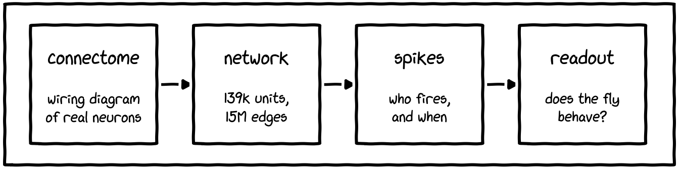
Figure 1. the four steps. the wiring diagram becomes a network, the network makes spikes, and the spikes tell you whether the fly acts right.
Two questions run in parallel. One is biological: if you poke the sugar-sensing neurons, does the simulated brain light up the same downstream cells a real fly does? The other is an engineering question: six tools, one network, do they agree, and which is fastest? Most of the code is about the second, which only means anything because the first one works.
why a whole fly brain, and why now
For a long time, computational neuroscience worked one circuit at a time. You modeled a handful of neurons you understood, because that was all the wiring anyone had. The map for anything bigger did not exist.
Connectomics changed the input. Slice a whole brain thin, image every slice under an electron microscope, trace every neuron and every connection, and you get a connectome. For the fruit fly that now exists: the FlyWire connectome, about 139 thousand neurons and roughly 54 million synapses, all reconstructed and labeled.
So the move this codebase makes is to stop modeling slices and simulate the whole thing at once, then check whether the complete network reproduces behavior the small models never could. Committing to a whole brain also changes what the hard part is. A few dozen neurons run instantly in any tool. A hundred and thirty-nine thousand of them, wired by fifteen million connections, turn the simulation itself into the engineering problem.
what are we actually simulating
A connectome tells you which neuron connects to which. Each connection also carries a strength, roughly how many synapses join the two neurons, and a sign. The sign comes from a separate prediction about each neuron’s neurotransmitter, made synapse by synapse from the electron microscopy images. GABA and glutamate count as inhibitory, acetylcholine as excitatory, and a neuron is called inhibitory when more than half of its outgoing sites are predicted that way. Sign and strength are multiplied together, so each connection ends up as one signed number.
The default experiment is called sugar, and it mirrors the fly’s feeding reflex. In a real fly, sugar-sensing neurons on the proboscis and legs detect something sweet, that signal runs inward, and a chain of neurons downstream ends in the muscles that extend the proboscis to feed. The readout is motor neuron 9, which extends the rostrum, the largest segment of the proboscis. The model forces the sugar-sensing neurons to fire and watches whether MN9 fires on its own.
It does, and the shape of the response matches the animal. Driving the sugar neurons on one side of the head produces a stronger response in the MN9 on the opposite side, which is what a fly does when it finds food with one leg: the proboscis extends and curves toward the source. Of the 127,400 proofread neurons in the paper’s connectome release, 45 respond to sugar input at 10 Hz and 455 at 200 Hz.
That list can be checked against decades of genetics. Ten cell types were already known to respond to sugar and to be sufficient for proboscis extension, and the model predicts all ten respond, with eight of the ten driving MN9. A harder test came from a screen of 106 cell types picked without regard to the model: eleven were predicted to drive MN9, ten of those eleven did when activated with light in a live fly, and of the remaining ninety-five, only four produced any extension. Across all 164 predictions the authors could test at the bench, 91 percent held, or 84 percent leaving that screen out.
what the model found
Two results show what a wiring diagram and two equations can buy. Neurons labeled by the receptor Ir94e respond to low salt, and the standing guess was that they made food more appealing. The model predicted the opposite, that driving them suppresses MN9 rather than exciting it. Shining light on those neurons in a live fly did suppress extension to sugar, which turned a hypothesis about attraction into a new aversive taste. The model also called the limit of that suppression correctly: strong Ir94e activity does not fully block a response to strong sugar, where bitter does.
The grooming circuit was the independent check, a system with no taste in it. Driving 147 mechanosensory neurons in the antenna, the model found four neurons capable of activating the descending neuron that triggers grooming, and three whose silencing reduced it. Those are the nodes years of genetics had already identified, and nothing spurious came along with them. It also caught a distinction nobody had predicted. Two classes of antennal neuron synapse onto the same interneuron at comparable strength, 103 synapses against 78, and only one of them actually drives it. Calcium imaging confirmed the split.
Sugar and water turn out to overlap heavily. At matched drive the sugar pathway lights up 377 neurons and the water pathway 391, with 250 shared between them, while sugar and bitter share exactly two. The overlap predicted something testable: silencing the sugar neurons should impair drinking, and it did.
the neuron: leaky integrate-and-fire
Every neuron in the network follows the same two rules. The first governs the voltage. Left alone, the voltage leaks back toward a resting level. Add some input and it climbs. The second governs the synaptic conductance, the running total of recent input, which decays toward zero.
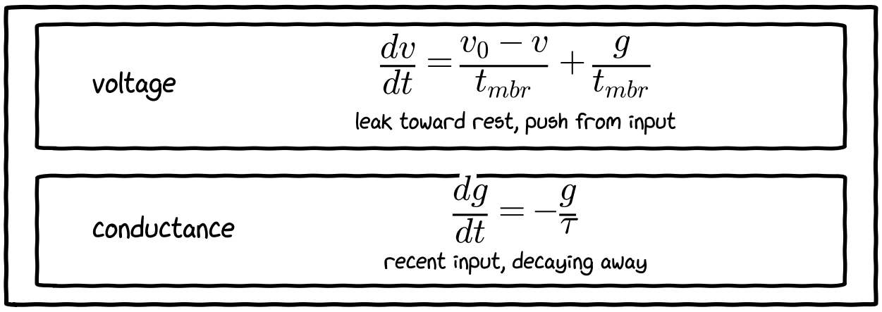
Figure 2. the two equations. the voltage moves back toward its resting value, and the conductance shrinks to zero over time.
If the first equation looks familiar, it should. It is a leaky capacitor: a neuron’s membrane holds charge like a capacitor and lets it leak like a resistor, and the product of the two sets how fast it forgets, which is the membrane time constant.
One sanity check makes the scale concrete. The voltage rests around -52 mV and fires at -45 mV, so a neuron has to climb about 7 mV to spike. No single input gets it there. It takes many, arriving close enough in time to stack up before the leak drains them away.
Two events interrupt that smooth drift. The first is a spike. When the voltage crosses the threshold, the neuron fires, and three things happen at once: the voltage snaps back to its reset value, the conductance clears to zero, and the neuron goes quiet for a 2.2 ms refractory period before it can respond to anything again.
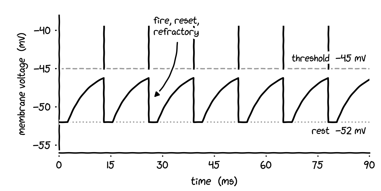
Figure 3. the voltage of one neuron. it rises until it hits the threshold, fires, drops back to rest, and waits before it can fire again.
The second event is a synapse delivering its input. When an upstream neuron fires, the conductance of each downstream neuron jumps by the weight of the connection between them, but not instantly: it waits out a fixed 1.8 ms delay, jumps, then fades away exponentially.
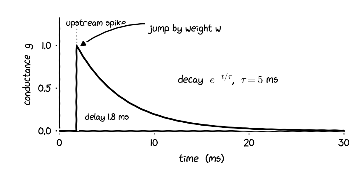
Figure 4. what one incoming spike does. after a short delay the conductance jumps up, then falls back down.
Why a fading conductance, instead of adding the weight straight to the voltage? Timing is the whole point. If every input landed instantly and vanished, two spikes arriving a little apart would count the same as two arriving together. The decay makes near-simultaneous input add up and spread-out input not. Most of what this network computes comes out of that difference.
The two variables drive each other in a loop. Spikes come in, wait out the delay, and land on the conductance. The conductance leaks into the voltage. The voltage gets checked against the threshold. Cross it and you get a spike out, plus a reset that clears everything and starts the wait again.
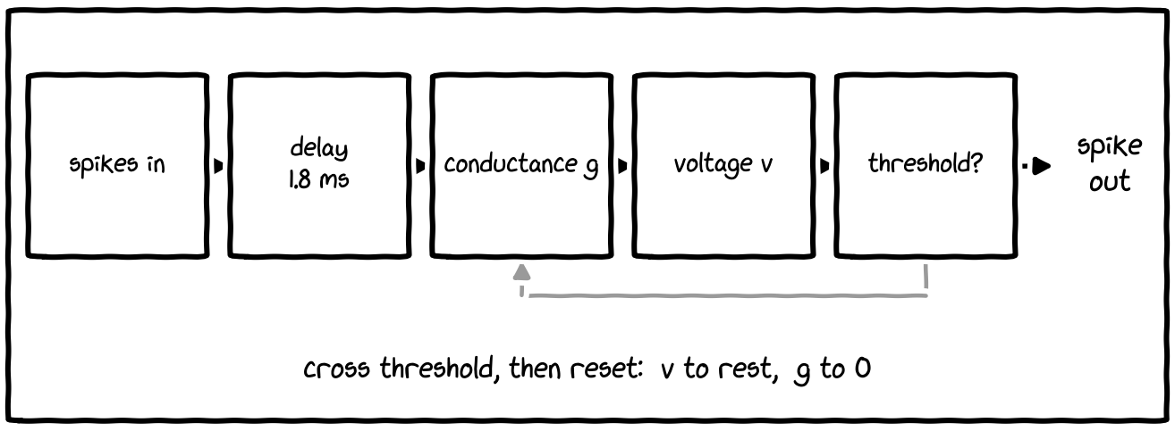
Figure 5. the same neuron drawn as a loop. when the voltage crosses the threshold it sends a spike and resets.
Every constant below comes from earlier fly modeling or from electrophysiology, and the code keeps the citation next to the value:
| symbol | value | what it is | source |
|---|---|---|---|
| v_0, v_rst | -52 mV | resting and post-spike reset potential | Kakaria & de Bivort 2017 |
| v_th | -45 mV | firing threshold | Kakaria & de Bivort 2017 |
| t_mbr | 20 ms | membrane time constant (R x C) | Kakaria & de Bivort 2017 |
| tau | 5 ms | synaptic decay time constant | Jurgensen et al. 2021 |
| t_rfc | 2.2 ms | refractory period after a spike | Lazar et al. 2021 |
| t_dly | 1.8 ms | delay from a spike to its downstream effect | Paul et al. 2015 |
| w_syn | 0.275 mV | voltage bump per unit of synaptic weight | free parameter |
| f_poi | 250 | scaling on the external Poisson drive | tuned to cause spiking |
Only w_syn is free, the voltage bump one unit of synaptic weight delivers. It was calibrated once, so that sugar neurons firing at 100 Hz drive MN9 to roughly 80 percent of its maximum rate, a target taken from feeding experiments. Everything else is measured. With almost nothing to tune, a result that matches the biology comes from the wiring rather than from a knob someone turned.
from a wiring diagram to a network
A connectome is a list of who connects to whom. To make it do something you need two more things: how strong each connection is, and what starts the whole thing moving. Strength is already in the table, as that signed weight per connection. The push that starts it comes from the input.
A sensory neuron fires at random moments, at some average rate. The model captures that with a Poisson process: for each stimulated neuron, spikes arrive randomly at a chosen average frequency. The rate comes from the experiment, so the sugar run and a walking run drive their own neurons at their own rates.
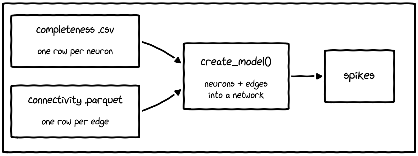
Figure 6. the two files become a network, and running it writes out spikes.
the two data files
Almost everything the model has about the fly sits in two files. The first is a CSV the code calls the completeness materialization, a list of neurons, one row each, indexed by FlyWire id. The second is the connectivity, stored as parquet because it is large and columnar reads are fast. Each row is one directed connection carrying the source index, the target index, and that signed weight.
What is absent: neuron shapes, dendrite geometry, spatial positions, per-synapse timing. In this model a neuron is a row and a connection is a single number.
Inside the simulator, neurons are numbered 0, 1, 2, by their row. Biology is keyed by FlyWire id instead. The code carries a map between the two, so results can be handed back to a biologist in ids they recognize.
the model, in seven lines
The file that builds the model takes the two tables and makes a network out of them. The neuron equations go in as written. The threshold, reset, and refractory rules go in as short expressions. Then the connections are made in bulk: the source and target index columns become the edges, and the weight column becomes the per-edge strength.
neu = NeuronGroup(N=len(df_comp), model=eqs, method='linear', threshold='v > v_th', reset='v = v_rst; g = 0*mV', refractory='rfc')syn = Synapses(neu, neu, 'w : volt', on_pre='g += w', delay=t_dly)syn.connect(i=df_con['Presynaptic_Index'].values, j=df_con['Postsynaptic_Index'].values)syn.w = df_con['Excitatory x Connectivity'].values * w_synThat is the entire network. The Poisson inputs get added on top for the stimulated neurons, any silenced neurons have their outgoing weights zeroed, everything is collected into one object, and it runs. Because each run is one random draw from the Poisson input, you never run it once. The model runs many trials, spreads them across CPU cores, and a short companion script averages each neuron’s firing rate across trials. Everything downstream compares against that firing-rate vector.
why simulate the same thing six ways
This is where a neuroscience model turns into a systems project. The model is fixed: same neurons, same weights, same equations. But a whole-brain spiking network is hard to run, and different tools make different trades to run it, so the codebase pushes the identical network through six of them and checks that they all land in the same place.
Every tenth of a millisecond of simulated time, all 139 thousand neurons update their voltage, and every neuron that just fired has to deliver its weight across all of its outgoing connections. The arithmetic per neuron is trivial, a couple of adds and multiplies. The cost sits in the delivery. Chasing fifteen million connections through memory, most of them to scattered addresses, is a memory problem rather than a math problem. A fly brain is therefore a good stress test for anything that claims to be fast.
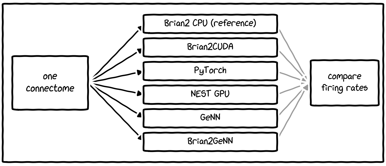
Figure 7. the same network run on six simulators. their spikes are compared against the Brian2 CPU result.
The six split into families. Two are Brian2 itself, once on the CPU and once on a GPU through Brian2CUDA. One is a hand-written PyTorch version that treats the whole network as tensors. Two are dedicated GPU spiking simulators, NEST GPU and GeNN. The last, Brian2GeNN, is a bridge that lets you write a normal Brian2 model but run it through GeNN’s code generator.
the six backends, one at a time
brian2 on the cpu: the reference
Everything else is measured against this one, and it stays closest to the original paper. It runs in two modes. For many trials it stays in Python and steps the simulation there, which is flexible. For long single runs it switches to standalone mode, where Brian2 generates C++, compiles it, and runs that instead. Those two modes are the benchmark’s whole question in miniature: interpret the model, or generate code for it.
brian2cuda: the same model on a gpu
Brian2CUDA is a Brian2 device that emits CUDA instead of C++. It reuses the exact network-building code from the CPU path, then targets the GPU and builds once. Only the hardware underneath changes.
pytorch: the network as tensors
The PyTorch backend is the most interesting of the six, because it drops the language of neurons and synapses and works entirely in tensors. Every neuron’s state becomes one big array. Those continuous equations turn into a plain forward Euler step at the same tenth-of-a-millisecond tick the others use. Brian2 handles the delay for you; here it becomes an explicit ring buffer: a small stack of recent inputs that shift forward one step at a time until they arrive.
The connectivity becomes a single sparse matrix, and delivering spikes becomes one sparse matrix-vector multiply per step. Take the current spike vector, multiply by the weight matrix, and every neuron’s fresh input arrives at once.
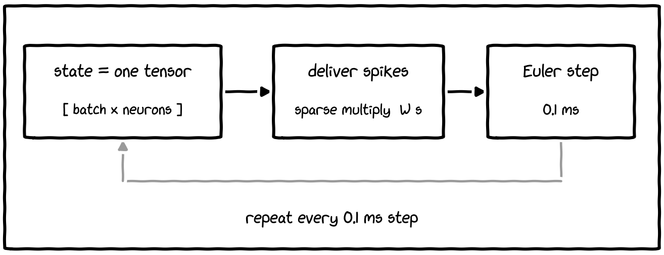
Figure 8. how PyTorch does it. the whole state is one big table of numbers, and each step is one matrix multiply.
Then the trick that pays for the GPU: the trials are batched. Instead of one trial at a time, the model stacks all of them along a batch dimension and runs them together, so a hundred trials cost barely more than one. The PyTorch code also carries a full surrogate-gradient setup, the trick that makes spikes differentiable so you could train the network, and never uses it.
nest gpu: a custom neuron, one subprocess per trial
NEST GPU is a purpose-built GPU simulator for spiking networks. The fly’s neuron is not in its standard library, so the codebase ships a custom one, written in CUDA and compiled in. There is a hard limit: NEST GPU cannot reset its state inside a running process. Once you have built and run a network, you cannot cleanly tear it down and start a fresh one in the same process. So every trial gets its own subprocess, which builds, runs, writes its spikes, and exits, and the parent merges the results.
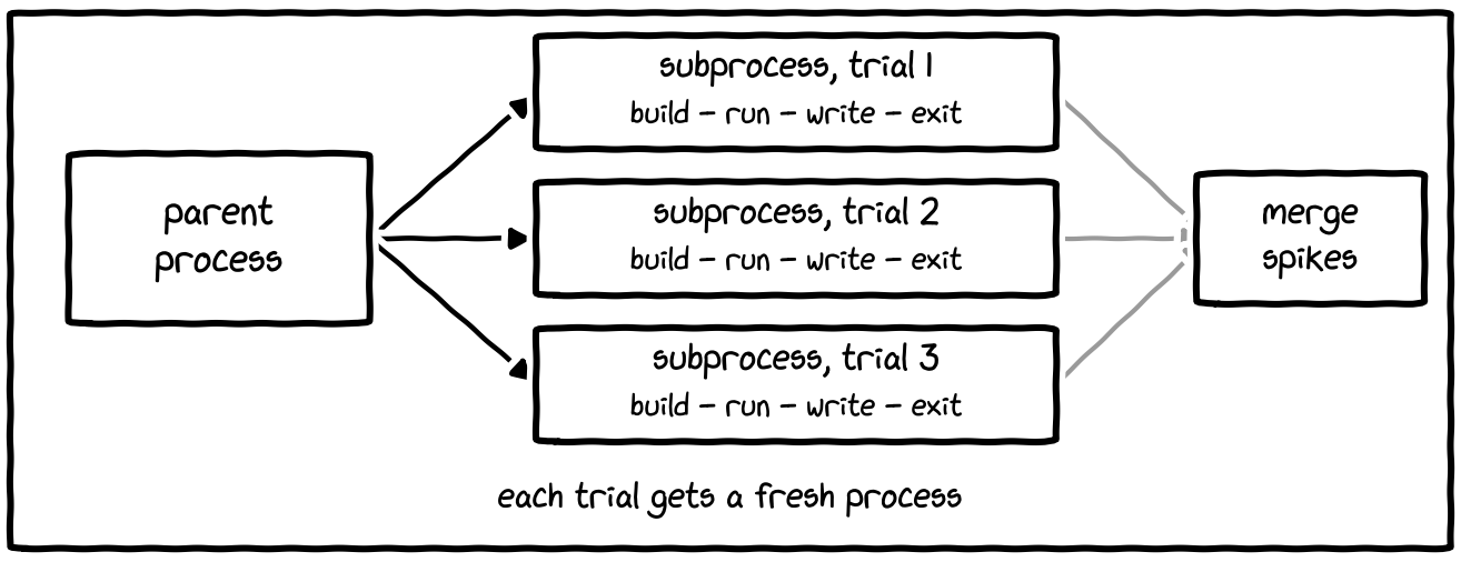
Figure 9. NEST GPU has to start a new process for every trial. the main process puts the spikes back together.
genn: generate the code for this exact network
GeNN takes code generation the furthest. Instead of interpreting a network, it generates CUDA source tailored to this specific model and compiles it. The runner defines the same custom neuron and a source model for the Poisson input, hands them to GeNN, and lets it build.
brian2genn: the bridge
Brian2GeNN lets you write an ordinary Brian2 model and run it through GeNN’s code generator, so you get GeNN’s speed while writing Brian2, and it lives in its own environment because it pins an older Brian2.
The six sit at six points on one axis. Brian2 CPU interprets the model. Brian2 standalone and Brian2CUDA generate code but keep Brian2’s structure. GeNN and Brian2GeNN generate code the whole way down.
making sure they all agree
Six versions are only useful if they compute the same thing. You cannot compare them spike for spike. The input is random, so the exact spike times differ every run, even from the same backend, and comparing timings directly would measure the randomness instead of the model.
What has to match is the firing rate. The input is random in its timing but fixed in its average rate, and the network’s response, averaged over enough trials, settles into a stable rate per neuron. So the comparison computes each neuron’s average firing rate in a backend, does the same for the Brian2 reference, and checks how well the two line up, using a plain correlation across neurons.
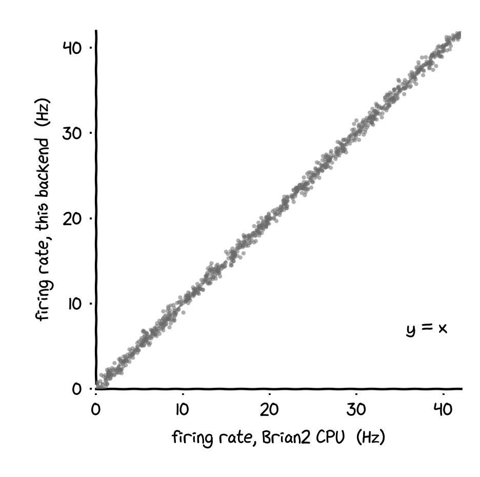
Figure 10. a good result. each dot is one neuron, and the dots sit on the line where both rates match.
Nothing about the order of operations, the hardware, or the random seed has to match, only which neurons fire and how hard. For a model driven by random input, no stronger promise is available.
the harness that keeps the numbers honest
A lot of this codebase is bookkeeping around the timings: crash isolation, what gets counted inside the timed section, and how a rerun overwrites its own row.
GPU simulators fall over in ways CPU code does not: a run can exhaust device memory, hang, or crash in a compiled kernel you did not write. The NEST GPU path treats every trial as something that might die, in its own subprocess, so one bad trial does not take the whole run down. Writing millions of spikes to disk takes seconds, and a pure speed comparison should not count that against the simulation, so the harness writes spikes outside the timed section.
Repeatability is handled by making the outputs safe to rerun. Timing results are appended to a CSV, but each row is keyed by the backend, the duration, the trial count, and the experiment, so rerunning updates a row instead of piling on duplicates. There is also plumbing for the environments this runs in, including GPU backends set up to work under Windows Subsystem for Linux, where the CUDA toolkit and a source-built simulator have to be found by hand.
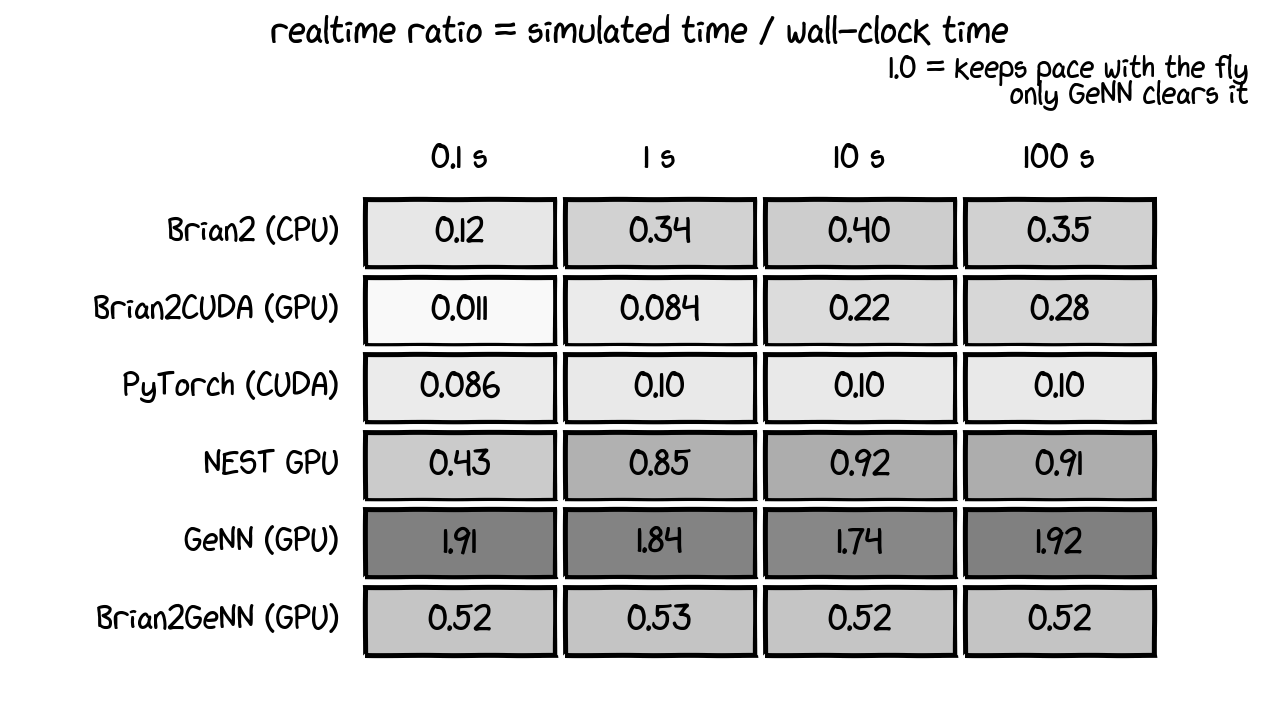
Figure 11. how fast each simulator ran. 1.0 means real time, and only GeNN is above it.
The headline metric is that realtime ratio, simulated time over wall-clock time. A ratio of one means the simulator keeps pace with the fly: one second of brain takes one second to compute. Above one, you are running the brain faster than it lives. Only GeNN gets there, at roughly 1.8 times realtime, and the ordering underneath it does not follow the CPU-to-GPU story you would expect: Brian2 on plain CPU beats Brian2CUDA on a GPU at every duration, and the PyTorch version, the one that looks most like modern machine learning, runs about a tenth of realtime.
how this was put together
Everything above came out of the repository before it came out of the paper. The code sits at github.com/eonsystemspbc/fly-brain: main.py parses the flags, code/benchmark.py dispatches to one runner per backend, and data/ holds the two connectome files. I worked through it in that order, writing down what each parameter did and tracing the equations out of the model file into all six runners, and went to the paper afterwards to check the biology against what the code was doing.
Reading in that order changes what is visible. The Nature paper describes one Brian2 implementation; the repository carries six, and the distances between them do not appear anywhere in the paper. NEST GPU spawning a subprocess per trial because it cannot reset in-process, PyTorch stacking trials into a batch dimension, Brian2GeNN living in its own conda environment because it pins Brian2 below 2.6 while Brian2CUDA wants 2.8.0: none of that is a scientific claim, and all of it is what running the model actually costs. The original paper code is in the repository too, under code/paper-brian2, sitting next to the refactor it became.
One difference only turns up in the data folder. The published results were computed on FlyWire materialization 630, and the repository runs on version 783, keeping 630 in data/archive purely for reproducing the paper’s figures. The connectome underneath this benchmark is a newer one than the connectome underneath the Nature numbers. What the paper supplied in return was the part no amount of source reading produces: which neurons were checked at the bench, how often the model was right, and which of its assumptions the authors already knew were wrong.
what stuck with me
Matching firing rates instead of spikes commits the code to the only thing a random model can guarantee, and it lets six wildly different implementations count as correct as long as their statistics agree.
A fly brain is a good benchmark for sparse, irregular, memory-bound work. There is no structure to exploit. The connectivity is whatever the fly’s wiring happens to be, and that kind of load separates hardware that looks fast on paper from hardware that is fast on a mess.
The unused surrogate-gradient apparatus in the PyTorch backend only turns up if you read the code. Someone left the door open to making this trainable and then did not walk through it.
Six simulators with totally different internals, from an interpreted Python loop to hand-written CUDA, all answer to the same firing-rate check. Whatever they do inside, they have to agree on the outside.
Every neuron is a single point with one voltage, no shape, no dendrites, no chemistry beyond a sign. Baseline firing is zero, so an inhibitory connection onto a silent neuron does nothing, and that single assumption accounts for the model’s clearest misses: two neurons that trigger extension in a live fly are predicted inhibitory and sit inert here. Gap junctions are absent for a harder reason, which is that electron microscopy cannot see them. And work on C. elegans and the crustacean stomatogastric ganglion showed long ago that one wiring diagram can support more than one circuit mechanism, so connectivity constrains a network without settling it. It should not work as well as it does. The fly runs the real version in real time, one second per second, on about a microwatt, while a desktop GPU barely keeps pace with the cartoon of it.
The model here is a refactor of the original Brian2 code Philip Shiu wrote for Shiu et al., A Drosophila computational brain model reveals sensorimotor processing, Nature 634, 210-219 (2024). The connectome is FlyWire.