Table of Contents
1. Overview
This project is a two-dimensional car simulation where a group of AI-controlled cars learn to drive around a race track without any human-written rules. There are no if-statements telling the car to turn when it sees a wall. There are no path-following algorithms. Instead, each car has a tiny neural network that reads sensor data and decides whether to steer left or right, and the weights of that network are shaped by an evolutionary algorithm over the course of many generations.
The algorithm used here is called NEAT, which stands for NeuroEvolution of Augmenting Topologies. It was introduced by Kenneth Stanley and Risto Miikkulainen in a 2002 paper, and the central idea is that you can train neural networks the same way nature trains organisms. You start with a population of random networks, you test them all in the same environment, you keep the ones that perform well, you let them reproduce with mutations, and you repeat. Over time, the population converges on networks that can actually do the task.
What makes NEAT different from other evolutionary approaches is that it does not require the network structure to be defined in advance. NEAT can add new connections and new neurons during the evolutionary process, starting from the simplest possible architecture and growing more complex only when it helps. In practice, this means the algorithm discovers not just the right weights but also the right shape for the neural network.
The simulation is written in Python using pygame-ce for the graphics and the neat-python library for the evolutionary algorithm. The full source code is available at:
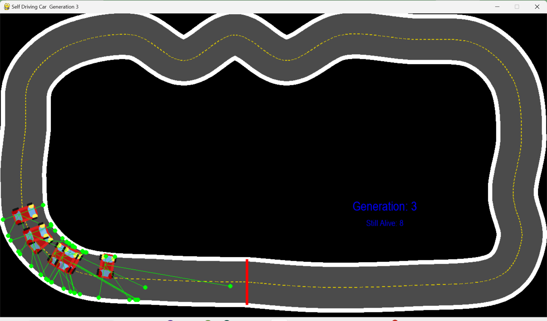
Figure 1: The final simulation. Thirty cars navigate curves and straights using only five distance sensors and a minimal neural network.
2. How the Car Perceives Its Environment
Each car in the simulation is equipped with five sensors. These sensors are raycasts, which is a common technique in game development where you extend an invisible line outward from a point and check what it hits. In this case, each ray starts at the center of the car and extends in a straight line until it reaches a white pixel (which represents a wall on the track) or reaches the maximum detection range of 300 pixels.
The five sensors are arranged at fixed angles relative to the direction the car is facing: 90 degrees to the left, 45 degrees to the left, straight ahead, 45 degrees to the right, and 90 degrees to the right. Together, they give the car a rough but sufficient picture of what is around it.
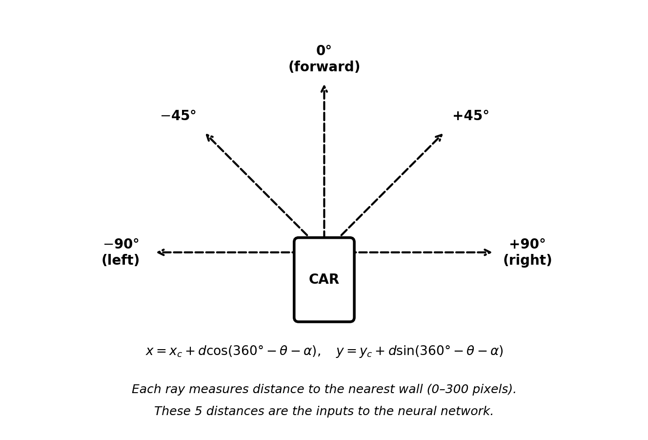
Figure 2: The five sensor rays extending from the car at fixed angles. Each one returns the distance to the nearest wall.
The raw distance values from each sensor can range from 0 (wall is touching the car) to 300 (nothing within range). To make these values easier for the neural network to process, each distance is divided by 30, which normalizes them into a range of roughly 0 to 10. This normalization step is important because neural networks tend to learn more reliably when their inputs are within a small, consistent range.
The underlying math for each sensor converts a polar coordinate (the car’s angle plus the sensor’s offset) into a Cartesian screen position. The formula for the endpoint of a ray at distance d is:
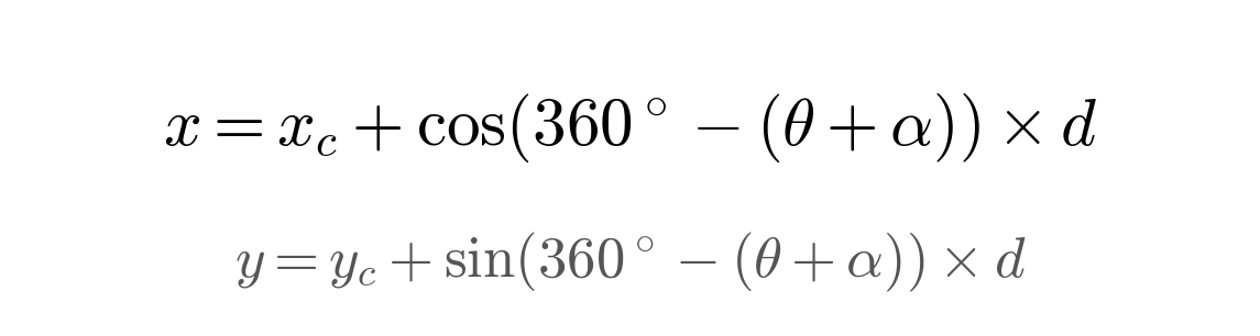
Figure 3: Converting a sensor angle to screen coordinates. The 360-degree subtraction corrects for pygame’s inverted Y-axis.
In this formula, x_c and y_c are the car’s center position, theta is the car’s current heading angle, alpha is the sensor’s angular offset (such as negative 45 degrees or positive 90 degrees), and d is how many pixels the ray has traveled. The reason for the 360-degree subtraction is that pygame uses a coordinate system where Y increases downward, which is the opposite of standard mathematical conventions. Without this correction, the sensors would point in the wrong directions.
3. The Neural Network
The brain of each car is a neural network. Neural networks are mathematical functions that take a set of input values, multiply them by learned weights, pass the results through a nonlinear activation function, and produce output values. In the context of this simulation, the inputs are the five sensor readings and the outputs determine the steering direction.
In the final working version of the simulation, the network architecture is as simple as it can possibly be. There are five input neurons (one per sensor), two output neurons (one for “steer left” and one for “steer right”), and zero hidden layers. This means that each sensor value is directly connected to each output through a weighted link, and the result is passed through the tanh activation function.
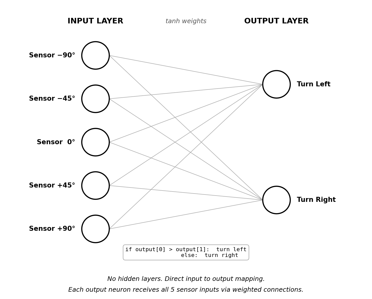
Figure 4: The neural network architecture. Five sensor inputs connect directly to two steering outputs with no hidden layers in between.
The decision logic is a straightforward comparison. If the value of the first output neuron is greater than the value of the second, the car turns left by 10 degrees. Otherwise, it turns right by 10 degrees. There is no speed control in the final version; the car always moves forward at a constant 8 pixels per frame. This means the network only needs to solve one problem: when to turn, and in which direction.
output = net.activate(car.get_data()) if output[0] > output[1]: car.angle += 10 # steer left else: car.angle -= 10 # steer right
The tanh function (hyperbolic tangent) is used as the activation function for all neurons. It takes any real number as input and compresses it into the range between negative one and positive one.
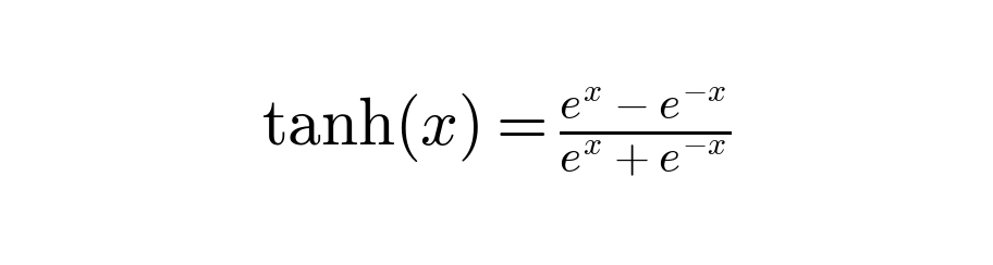
Figure 5: The tanh activation function. It maps any real-valued input to a bounded output in the range [-1, 1].
This compression is useful because it prevents the network from producing arbitrarily large output values, which helps keep the training process stable.
4. Measuring Performance: The Fitness Function
Evolution needs a way to tell which individuals in a population are performing well and which are not. This is the role of the fitness function. It assigns a numerical score to each car at the end of its life, and that score determines how likely the car’s neural network is to be passed on to the next generation.
The fitness function used in this project is:
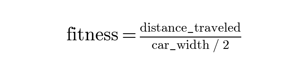
Figure 6: The fitness function. Distance is accumulated every frame and normalized by half the car’s width.
Every frame that a car remains alive, it is moving at 8 pixels per frame, and that distance adds up. A car that survives for 10 seconds (600 frames at 60 fps) will have traveled about 4,800 pixels, giving it a fitness of around 240. A car that crashes into a wall after just 2 seconds gets a fitness closer to 48.
What is notable here is how little information this function provides. There is no reward for staying in the center of the road, no penalty for wobbling back and forth, and no instruction to follow the track in any particular direction. The only feedback is: the further you drove before hitting something, the better your score. Despite this simplicity, it turns out to be enough for the population to converge on smooth, effective driving behavior within a small number of generations.
5. The Evolutionary Process
After each generation ends (which happens either when all thirty cars have crashed or when forty seconds have elapsed), NEAT evaluates everyone’s fitness scores and produces the next generation. This cycle follows a pattern that closely mirrors biological natural selection.
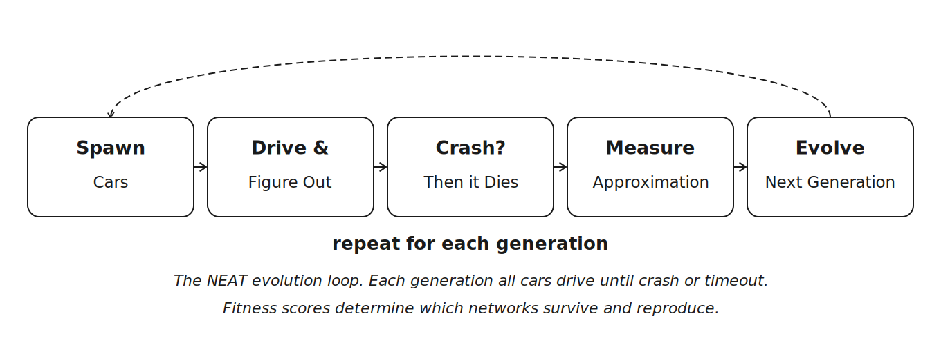
Figure 7: The evolution cycle. Spawn the population, let them drive, measure fitness, apply selection and mutation, repeat.
**Selection. **Cars are ranked by fitness. The ones that drove the furthest are the most likely to contribute their genes to the next generation.
**Elitism. **The top two performers are copied directly into the next generation without any modification. This is important because it guarantees that the best solution discovered so far cannot be lost due to random mutation.
**Reproduction with mutation. **Surviving networks produce offspring by copying their weights with small random perturbations applied. The main mutation adjusts each connection weight by a small random value:
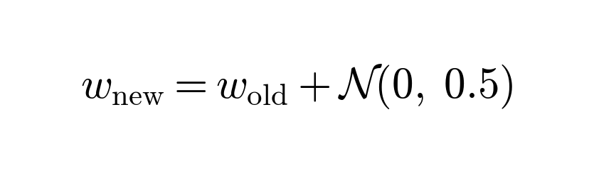
Figure 8: The weight mutation formula. Each weight is nudged by a random value drawn from a normal distribution.
Because the random value comes from a bell curve centered at zero, most mutations are small. Occasionally a larger change occurs, which can push the network into a new region of the solution space. There is also a 50 percent chance per generation of adding a new connection between neurons, and a 20 percent chance of inserting a new hidden neuron into the network.
**Speciation. **NEAT groups networks that have similar structure into species. Networks within the same species only compete against each other, not against the entire population. This protects newly evolved structures from being immediately eliminated by older, more optimized competitors. The grouping is based on a compatibility distance formula:
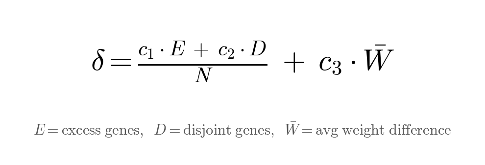
Figure 9: The NEAT compatibility distance. E counts excess genes, D counts disjoint genes, and W-bar is the average weight difference of matching genes.
If the compatibility distance between two networks is less than 3.0 (the threshold used in this project), they belong to the same species. If a species shows no improvement in fitness for 20 consecutive generations, it is removed entirely.
6. The Track and Project Structure
The simulation runs in a window of 1280 by 720 pixels. The track is stored as a PNG image where the white pixels represent walls and the gray area is the drivable road surface. The black region inside the track loop also counts as a wall, so the car is effectively confined to the gray corridor between the inner and outer white borders.
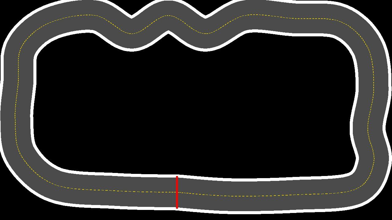
Figure 10: The race track. White borders define the collision boundaries. The red line marks the starting position.
The entire project consists of four files: car_simulation.py (the main simulation code, including the Car class, sensor logic, game loop, and NEAT integration), config.txt (all NEAT configuration parameters, including population size, mutation rates, and species thresholds), map.png (the track image — white pixels are walls, gray is the drivable surface), and car.png (a small top-down car sprite, 40 by 60 pixels).
All thirty cars spawn at position (400, 625) facing to the right. Collision detection works by calculating four corner points of the car’s bounding rectangle using trigonometry, and then checking whether any of those corners land on a white pixel. If even a single corner touches white, the car is considered crashed and is removed from the active simulation.
7. Development Process
7.1 Environment Setup
The development environment was a Windows 10 machine with Python 3.14 installed. The standard pygame package did not support this Python version at the time, so the pygame-ce (Community Edition) fork was used instead. This fork is maintained by the pygame community and provides support for newer Python releases. The two required packages were installed with a single command:
python -m pip install neat-python pygame-ce
7.2 Starting Simple: The Oval Track
The first version of the simulation used a simple oval track with wide, gentle curves. The goal at this stage was to verify that the basic components worked correctly: that the cars could spawn, that the sensors returned meaningful values, that the neural networks received the right number of inputs, and that the evolutionary loop ran without crashing.
Three bugs came up during this initial phase. The NEAT configuration required a parameter called no_fitness_termination that was not included in the first version of config.txt. The sensor code threw an index error when a ray extended past the edge of the screen, because it tried to read a pixel at coordinates outside the image bounds. And the cars were spawning on top of a white border pixel, which meant every single car died on the first frame of every generation.
After fixing these issues, the cars learned to navigate the oval track in a single generation. The track was simply too easy. Because the oval only curves in one direction, the only skill a car needs is to consistently favor one turning direction when it detects a wall. Even a completely random neural network has a reasonable chance of stumbling onto that behavior.
7.3 Increasing the Difficulty
The next step was to replace the oval with a more challenging track that included zigzag sections, chicanes, and sharp corners. This is the track shown in Figure 10. The increased complexity revealed a problem that would persist for many iterations of the project.
The population consistently got stuck at the first sharp right-hand turn. For over a hundred generations, every car in every generation would crash at the exact same point on the track. This behavior is an example of what is called a local optimum: the fitness function rewarded total distance, and cars that drove fast on the opening straight scored higher than cars that drove cautiously. Because the high-fitness parents were all fast, straight-line drivers, their offspring inherited the same tendencies. Over time, the entire population converged on a strategy of driving as fast as possible in a straight line, which is locally optimal on the straight section but completely fails at the first turn.
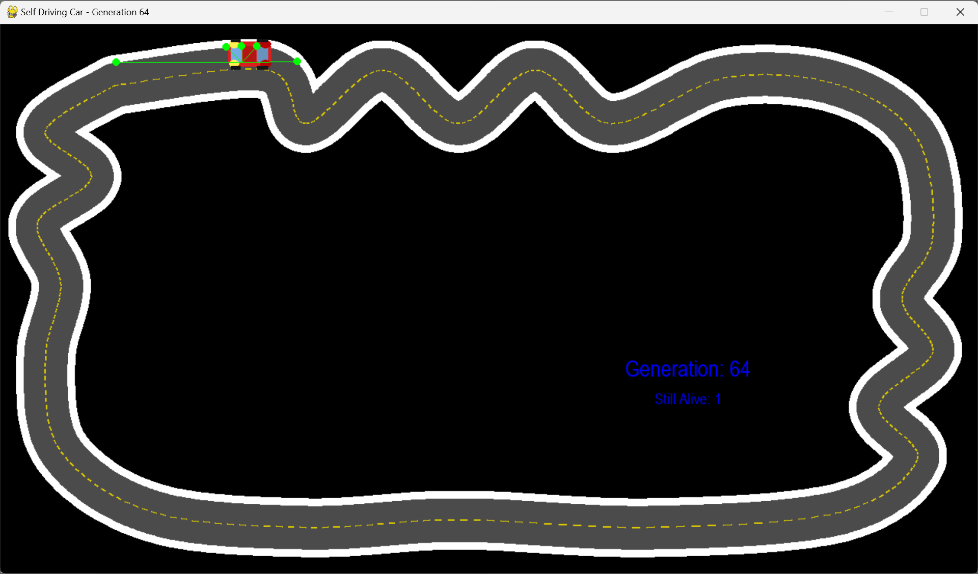
Figure 12: Generation 64. The last surviving car is stuck at the entrance to the zigzag section. This pattern repeated for over a hundred generations.
The core issue was a lack of genetic diversity. Once the population converges on a single strategy, there are no alternative approaches left in the gene pool to draw from. The mutation rate was not high enough to spontaneously generate a turning-capable network from a population of straight-line specialists.
7.4 Adding Complexity (and Making Things Worse)
The natural response to the stuck problem was to give the cars more information and more tools. Over several iterations, the simulation accumulated a number of additional features: the sensor count was increased from five to nine with a denser forward cluster, a third output neuron was added to control speed (allowing the network to slow down for turns), numbered checkpoints were placed around the track with large fitness bonuses for reaching each one, a time-to-live timer was added to kill cars that did not make forward progress, and the mutation rate was set to increase dynamically when the population stagnated.
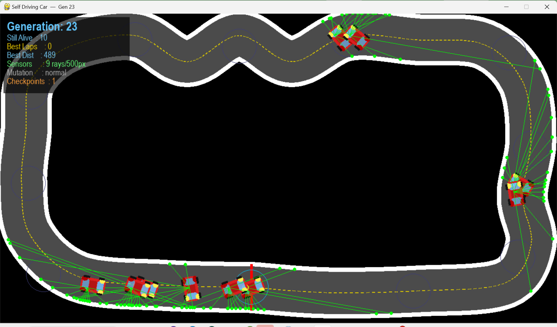
Figure 13: The overcomplicated version. Nine sensors, three outputs, checkpoints, and mutation boosting, all running at once.
Each of these additions introduced its own set of bugs and unintended consequences. The checkpoint system caused a cascade failure where cars spawned directly on top of the first checkpoint, triggered it immediately, and then died before reaching the second one, resulting in every car dying on frame zero. The speed control output gave the network a new way to exploit the fitness function by simply driving slowly and surviving longer without actually making progress around the track. The multiple spawn points that were tested caused some cars to discover that driving backward along a straight section was the safest available strategy, because a backward-driving car could survive for 7.5 seconds on a straight while a forward-driving car crashed at the first turn in under 3 seconds.
7.5 The Key Insight: Simplification
The turning point of the project was the realization that every feature that had been added to help the cars learn was actually making the problem harder for the evolutionary algorithm to solve. More sensors meant more input dimensions for the network to process. Speed control meant the network had to optimize two behaviors (steering and throttle) simultaneously instead of one. Checkpoints and time-to-live introduced complex interactions and edge cases that interfered with the core learning signal.
The solution was to strip the simulation back to its absolute minimum. The final version uses five sensors, two output neurons, no hidden layers, a fixed speed of 8 pixels per frame, and wall collision as the only termination condition. There are no checkpoints, no time-to-live timer, no speed control, no dynamic mutation, and no multiple spawn points.
Removed features and why removing them helped: Speed control (third output neuron) — reduced the problem to a single optimization target: steering. Hidden layers — a direct 5-to-2 mapping requires far fewer generations to train. Checkpoints and TTL — eliminated an entire class of edge-case bugs and exploit paths. Multiple spawn points — removed the backward-driving exploit. Extra sensors (9 down to 5) — reduced input noise without losing meaningful information.
After making these changes, the simulation started working reliably. Cars learned to navigate the full track within 5 to 15 generations, and the learning was consistent across repeated runs. The simplified architecture actually outperformed every complicated version that preceded it.
Figure 14: The final simplified version. Cars consistently learn to handle curves and straights within a few generations.
8. Implementation Details
8.1 Frame-Zero Initialization
One subtle but important bug appeared early in development. The NEAT library calls the neural network’s activate function on every frame, including the very first frame of each generation. However, on frame zero, the car has not yet run its update loop, which means the sensors have not been calculated. Passing an empty list of sensor values caused a RuntimeError because the network expected exactly five inputs.
The fix was to initialize five placeholder sensor values in the Car constructor, so that the network always has something to work with:
self.radars = [ [(int(self.center[0]), int(self.center[1])), 1] for _ in range(5) ]
These values are overwritten on the next frame when the actual sensors run. The placeholder ensures that the simulation does not crash before it gets a chance to start.
8.2 Collision Detection
The car’s shape is approximated by four corner points placed at 30 and 150 degrees (and their negatives) from the car’s heading, at a distance of half the car’s width from the center. On every frame, each corner’s screen coordinates are calculated and checked against the track image:
for point in self.corners: x, y = int(point[0]), int(point[1]) if x < 0 or x >= WIDTH or y < 0 or y >= HEIGHT: self.alive = False return if game_map.get_at((x, y)) == BORDER_COLOR: self.alive = False
If any corner lands on a white pixel or goes outside the window boundaries, the car is marked as dead and stops participating in the simulation for the remainder of that generation.
8.3 Configuration Reference
The NEAT configuration file controls every parameter of the evolutionary process. Key parameters in the final version: num_inputs=5 (one input neuron per sensor ray), num_outputs=2 (steer left vs. steer right), num_hidden=0 (no hidden layers in the initial network topology), pop_size=30 (number of cars spawned per generation), elitism=2 (top two performers copied unchanged to next generation), weight_mutate_rate=0.8 (probability that each weight is mutated), weight_mutate_power=0.5 (standard deviation of Gaussian noise added to weights), conn_add_prob=0.5 (probability of adding a new connection per generation), node_add_prob=0.2 (probability of adding a new hidden neuron per generation), compatibility_threshold=3.0 (maximum distance for two genomes to be in the same species), max_stagnation=20 (generations without improvement before a species is removed), activation=tanh (activation function used for all neurons).
9. Takeaways
The most significant lesson from this project is about the relationship between problem complexity and solution complexity. When the evolutionary algorithm was struggling, the instinct was to give it more tools, more sensors, more outputs, more sophisticated fitness functions. In reality, each of those additions expanded the search space and made it harder for the algorithm to find a good solution. The breakthrough came from going in the other direction entirely, from reducing the problem to its simplest possible form and letting the algorithm work on a version of the task where even a minimal network could succeed.
The second lesson concerns fitness function design. The fitness function is the sole channel of communication between the designer and the evolutionary process. Everything the algorithm knows about what constitutes good driving behavior comes from the fitness score. When the fitness function was poorly designed (for example, rewarding survival time without distinguishing between forward and backward motion), the population exploited the loophole perfectly. The algorithm was not broken; it was doing exactly what it was told. The problem was always in the specification.
A third, more practical lesson is that initial conditions matter more than they seem to in a simulation like this. At least four separate bugs during the development of this project traced back to the car’s spawn position, spawn angle, or uninitialized sensor values. When something is not working in a simulation, verifying the starting state should be the first debugging step before making any changes to the algorithm itself.
10. Running the Simulation
To run the simulation, clone the repository and install the required packages:
git clone https://github.com/sandesh-8622/NEAT-self-driving-car cd self-driving-car-neat pip install neat-python pygame-ce python car_simulation.py
The simulation window shows the current generation number and the count of cars still alive. Green lines extending from each car are the sensor raycasts, which can be helpful for visualizing what the network is responding to. Press Escape at any time to quit.
To create and use a custom track, draw a 1280 by 720 pixel PNG image with white borders around the edges of the road. Save it as map.png in the project directory and update the SPAWN_X, SPAWN_Y, and SPAWN_ANGLE constants at the top of car_simulation.py to place the cars on a valid road position facing the correct direction.
11. References
Stanley, K.O. and Miikkulainen, R. (2002). “Evolving Neural Networks through Augmenting Topologies.” Evolutionary Computation, 10(2), pp. 99-127.
neat-python library documentation: https://neat-python.readthedocs.io
pygame-ce (Community Edition): https://pyga.me
Source code: https://github.com/sandesh-8622/NEAT-self-driving-car
Sandesh Bhandari, 2026