Table of Contents
If you are reading this, you probably think the hard part of using a thousand GPUs is the code. You have seen the diagrams of data, tensor, and pipeline parallelism, and you have heard about all-reduce collectives and sharded optimizers; the whole thing has the feel of a deep engineering problem that only a handful of elite labs have truly solved. So when a project needs to scale, the instinct is to hire the parallelism wizard, the person who can wire the model across the cluster and make the GPUs talk without deadlocking.
I think that instinct gets the problem backwards. Splitting a model across GPUs, for the cases most people actually face, is close to solved: the recipes are published, the libraries are mature, and the efficiency has settled into a narrow band. That part is paved. What is not solved, and what really decides whether your thousand GPUs were worth owning, is keeping them full. That is not a kernel problem. It is a demand problem.
Here is the constraint underneath all of it. A GPU is a fixed cost pretending to be a variable one. You pay for the whole chip, all the time, whether it is computing or sitting idle, so the only number that ever matters is the fraction of the chip you actually use, and that fraction is bought with demand, not with code. The layout decides whether you can reach the ceiling. Demand decides whether the ceiling was worth buying. Once you see scaling this way the parallelism stops looking like the interesting part, and two dull questions, how much work do I really have and how steadily does it arrive, turn out to decide almost everything.
the engineering is a paved road
Start with the part everyone treats as hard, because it is the part that is mostly done. There are three ways to spread a model across GPUs and they compose. Data parallelism puts a full copy of the model on every GPU, feeds each copy a different slice of the batch, and averages the gradients at the end. Tensor parallelism splits a single matrix multiply across several GPUs so each holds a shard of the same layer. Pipeline parallelism cuts the model into stages along its depth and streams microbatches through them like parts down an assembly line. You choose a rectangle of these three to fit your model and your network, and that is all there is to it.
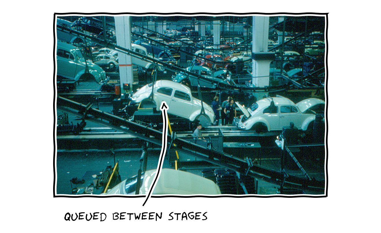
Wolfsburg, 1960. Car bodies moving from one station to the next.
It feels solved because the published numbers stopped surprising anyone years ago. When a trillion-parameter model was trained across a few thousand GPUs, the weak-scaling results ran from a 1.7-billion-parameter model on 8 GPUs up to a one-trillion-parameter model on 3,072, and the striking thing is not the size. It is how little the per-GPU efficiency moved across that whole range. One caution before the chart, because I lean on a stricter number later: what is plotted is throughput as a fraction of the chip’s peak, which counts every floating-point operation the hardware ran, including the ones spent recomputing activations to save memory. It is the friendly measure of how busy the silicon was. The harsher one comes in two sections.
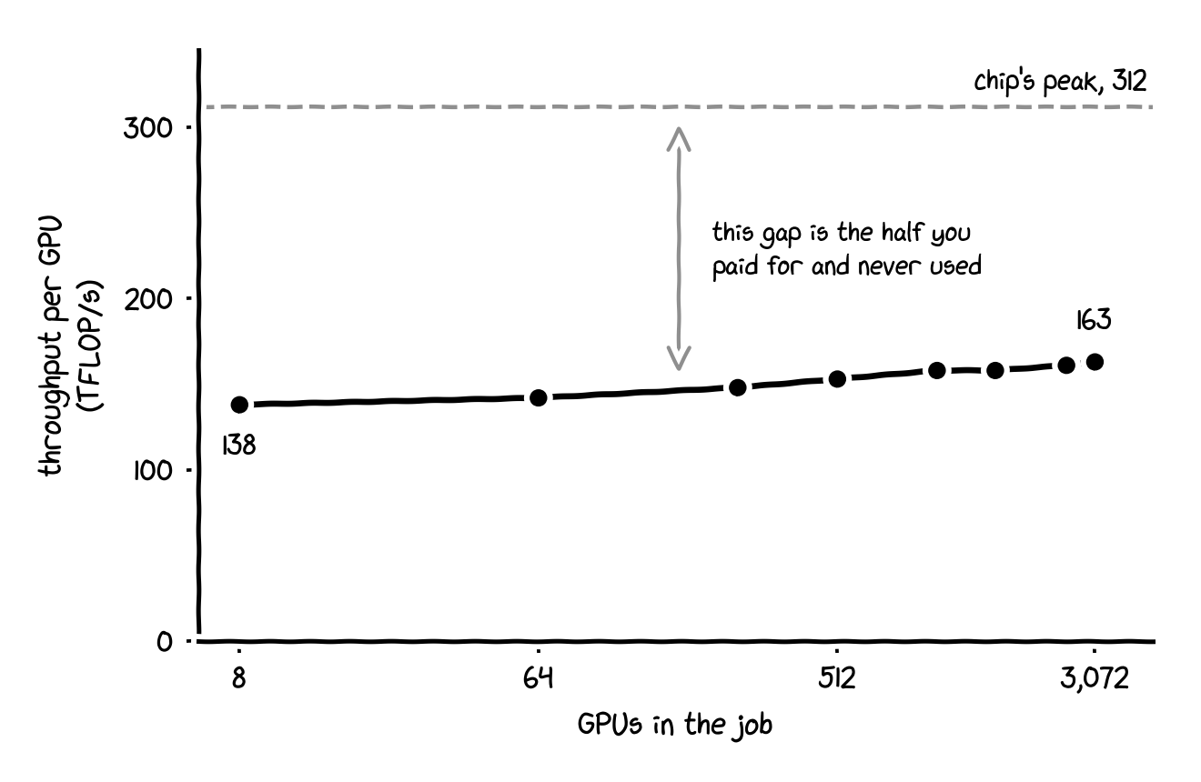
Figure 1. speed per GPU barely moves from 8 GPUs to 3,072.
The small model on 8 GPUs ran at about 138 teraFLOP/s per GPU, roughly 44 percent of the chip’s theoretical peak. The trillion-parameter model on 3,072 GPUs ran at about 163 per GPU, roughly 52 percent. You multiplied the machine by 384 and the per-chip throughput went up rather than down. That is near-perfect weak scaling, and it is remarkable in the way a paved road is remarkable: someone did the hard work once, and now you drive on it.
why there is essentially one good layout
That convergence is not luck, and the reason is physical. Each kind of parallelism communicates differently, and where each one is allowed to live is set by how fast a link it needs. Tensor parallelism is the hungry one: splitting a single matrix multiply means the GPUs have to exchange and sum partial results inside every layer, once in the forward pass and again in the backward, right in the hottest part of the computation. That only works if the chips share the fastest interconnect there is, so tensor parallelism belongs inside a single server where the GPUs are wired directly together. Pipeline parallelism is more relaxed, because it only passes a batch of activations across a stage boundary a few times per step, so it tolerates the slower links between servers. Data parallelism is the most relaxed of all: each replica runs on its own data in the forward pass, and the only thing that has to be combined is the gradients, once per step, in a single all-reduce at the end.
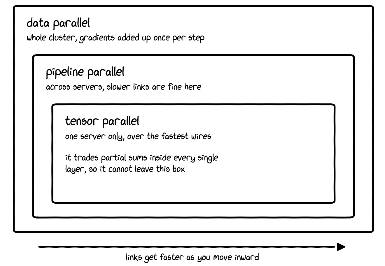
Figure 2. each split sits where the wires are fast enough for it.
| splits | communicates | how often | where it lives | |
|---|---|---|---|---|
| data | the batch | gradients, one all-reduce | once per step | outermost, across the cluster |
| pipeline | the model's depth | activations at stage edges | a few times per step | across servers, slower links ok |
| tensor | a single matmul | partial sums, all-reduce | inside every layer | one server, fastest link only |
So the order falls out on its own. Tensor parallelism on the inside where the wires are fast, pipeline parallelism spanning servers, data parallelism on the outside synchronizing once a step. There are not many good configurations because the hardware does not leave room for many, and when a lab publishes its training stack the design is rarely novel, because there is barely room for it to be. It is the configuration the interconnect forces on you, implemented carefully.
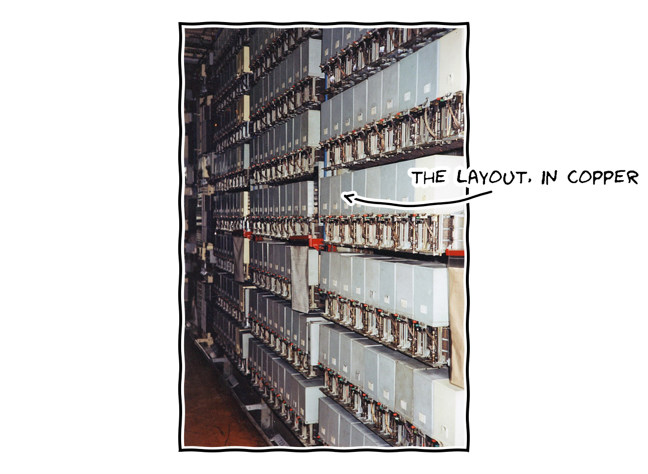
A telephone exchange. The wiring is the design.
I should be honest about where that stops being true, because the claim of one good layout has real edges and a careful reader will know them. The clean story assumes a dense model whose layers fit the tensor-inside, pipeline-across, data-outside nesting. Mixture-of-experts models break it head on: the experts are scattered across the cluster and every token has to be routed to the few it needs, which turns the hot path into an all-to-all shuffle over the network rather than a tidy all-reduce inside a server, and keeping that traffic balanced is a live problem, not a settled recipe. State-space models change the shape of the sequence dimension and with it how you split a long context. A cluster wired with ordinary ethernet instead of a fast fabric loses the very assumption that lets tensor parallelism exist. Runs that cross into the tens or hundreds of thousands of GPUs meet failure rates and communication patterns the published recipes never had to handle. And any genuinely new architecture has to find its own layout from scratch. So the paved road is real, but it is the road through familiar country. Off it, the engineering is the problem again, and those are exactly the places a parallelism expert earns the title. For the dense model on an ordinary cluster that most teams actually run, the road is paved, and that is the case the rest of this is about.
peak flops is marketing; utilization is the bill
The number the marketing deck wants you to look at is peak FLOPS. The number that decides whether the cluster was a good idea is utilization, the fraction of that peak you turn into useful work, and the two are not close. Here is the stricter measure I promised. Model FLOPs utilization counts only the operations your model mathematically requires, the ones that would appear in the math even on perfect hardware, divided by what the chip could have done in the same wall-clock time.
That is a harder test than fraction-of-peak, because it throws out the recomputation and the overhead and credits you only with work the model actually needed. It is why the figures here sit below the 44 to 52 percent from the weak-scaling chart: the same runs, counted more strictly. And under that accounting, even the best training runs in the world come out low.
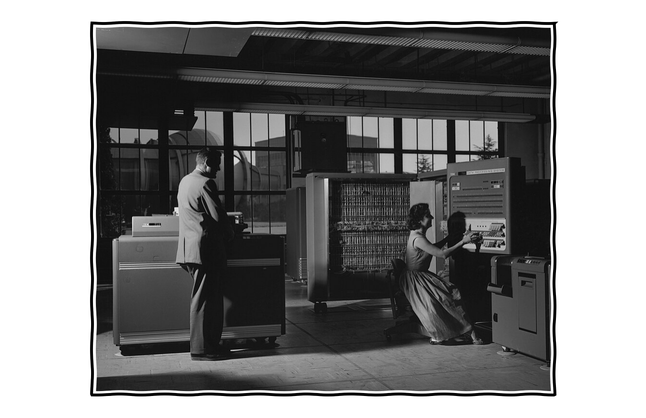
NASA, 1958. Computer time cost so much that keeping the machine busy was someone’s whole job.
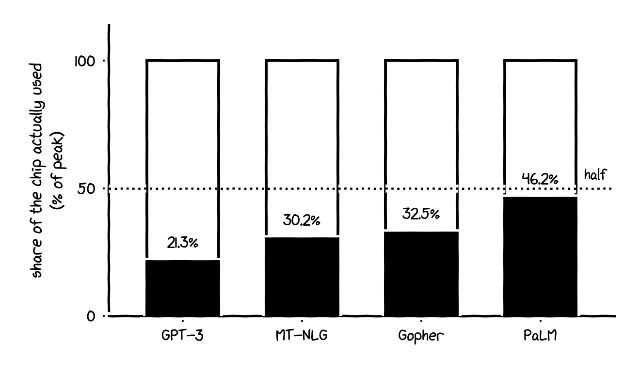
Figure 3. even the best public run leaves over half the chip idle.
One landmark model ran at about 21 percent. A 530-billion-parameter joint effort managed about 30, and another large model reached about 33. The best of them, engineered hard for utilization with a custom layout and an aggressive compiler underneath, reached about 46 percent, and that was treated as a triumph. The best-resourced teams in the world, optimizing for exactly this, used under half the silicon they paid for. The lesson does not stay inside training. You can build a chip with enormous peak FLOPS, but if you cannot feed it the peak is a fiction; we are very good at producing FLOPS and bad at keeping the arithmetic units fed, and at the cluster level the same problem repeats one rung up, where the hard part is keeping the GPUs fed with work. Utilization is the name for how well you are doing that, and it is the only efficiency number that survives contact with a finance spreadsheet.
a gpu is a fixed cost pretending to be a variable one
Here is the economic fact the engineering framing hides. When you buy or rent a GPU you pay for the device, not for the computation. A rented chip costs the same per hour whether it runs at 60 percent utilization or 6. An owned one costs its purchase price spread over its life, plus power and cooling and the slot in the building, and that bill arrives on a schedule that has nothing to do with how busy the chip was. The FLOPS are not metered. The clock is.
A chartered plane is the cleanest version of the idea. Once you have chartered it the cost of the flight is fixed, and whether you fill every seat or fly it empty you pay the same, so the cost per passenger is not a property of the plane. It is a property of how many passengers you found. A full flight is cheap per head and an empty one is ruinous, and the plane is identical in both. A GPU works the same way, and the seats are the slots in its compute and memory that a unit of work can occupy.
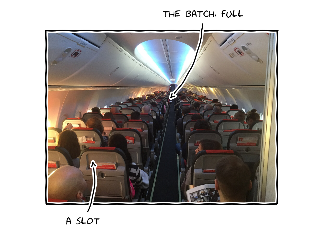
A full flight. The plane costs the same to fly either way.
Your cost per useful operation is the hourly bill divided by the useful operations you got out of that hour. Double the useful operations and you halve the unit cost on the same chip, the same power, the same depreciation; halve them and you double it. The hardware never changed, only the fullness did. Which is why adding GPUs does not add value, it adds fixed cost, and the value appears only if the new chips are full. Whether they are full has nothing to do with how elegantly you sharded the model and everything to do with whether you brought enough work to occupy what you bought. The parallelism library will happily spread your job across all thousand chips. It cannot tell you whether you should have.
where the fullness actually comes from
Now I can be concrete about where utilization comes from, and it is here that the word economics earns its place, because the lever is demand. The clearest case is inference, where most GPUs spend most of their lives and where the fixed-cost trap bites hardest. A language model generates text one token at a time, and producing each token requires reading the entire model’s weights out of memory. Serve a single user and you read all those weights, do a tiny amount of arithmetic for that one sequence, and throw the read away, so the arithmetic units sit nearly idle while the memory system does all the work. There is a precise way to name what is wrong. Every workload has an arithmetic intensity, the number of operations it does for each byte it moves from memory, and a chip can only approach its peak once that intensity is high enough. Single-stream decoding sits far below the line where compute even becomes the limit.
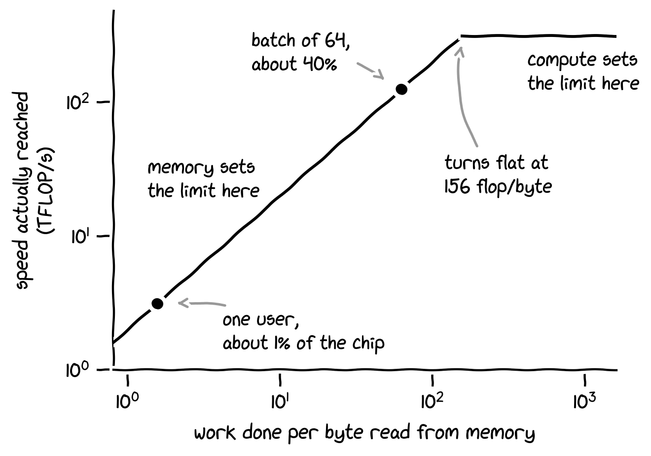
Figure 4. one user starves the chip. a full batch walks it up the roof.
The fix is batching: serve many users at once so that one expensive read of the weights is shared across many sequences. The reads stay roughly fixed while the useful arithmetic multiplies, the intensity climbs, and the chip finally has something to do. The size of the effect is not subtle. The same accelerator can produce on the order of twenty-seven times more tokens per second at a batch of 64 than at a batch of 1, and nothing about the chip changed; you did not overclock it or add memory, you filled it. As raw utilization, a single-stream decode can sit near 1 percent of the chip’s capability while a well-fed one tops out near half, and the factor between those two states dwarfs anything a kernel can hand you.
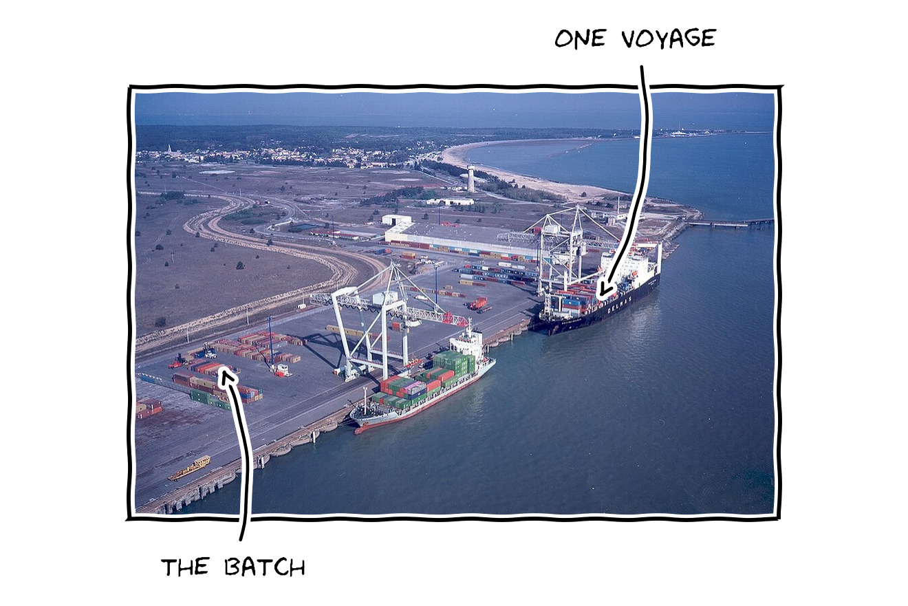
One ship, thousands of containers splitting the cost of the trip.
Two limits, both living in memory, decide how far this goes, and it is worth stating them as a clean pair. Bandwidth caps how fast you can read the weights, which sets the floor on intensity and is the thing batching fights against. Capacity caps how many sequences you can hold at once, because each one carries its own growing cache of keys and values in the same memory as the weights, so past a point the batch simply cannot grow. The first bound is why a lone request is slow. The second is why you cannot always batch your way out of it. Much of the serious engineering in inference is really memory engineering aimed at these two: packing that key-value cache so it wastes less room, and splitting the bulk prefill of a prompt from the one-token-at-a-time decode onto separate hardware so neither starves the other.
utilization is attracted, not engineered
This is the hinge of the argument. To fill a batch you need concurrent requests, and concurrent requests are a user base, so utilization is not something you engineer. It is something you attract. A model with a million simultaneous users keeps its batches full without trying and runs near the efficient end of the range. The identical model with a hundred sporadic users runs near the empty end, on identical hardware, at many times the cost per token. The temptation is to go hunting for the inference trick that closes that gap, but the gap is usually not a software defect. It is an absence of demand.
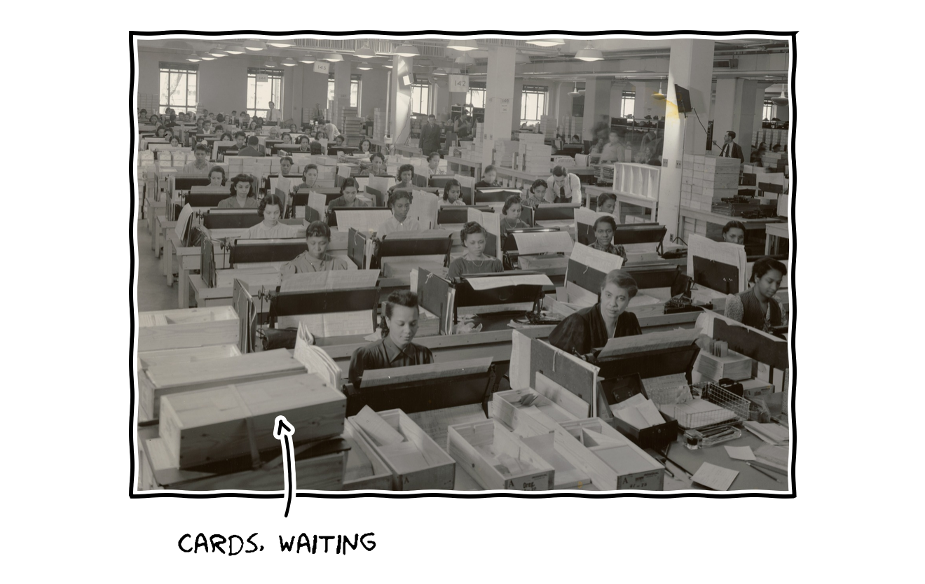
The 1940 census. 328 million cards punched by hand to keep the machines fed.
The economics sharpen when demand is uneven, because real traffic is spiky. A workload that arrives in bursts underfills its batches most of the time and briefly overflows them, and across a day it can run three to five times worse than the clean peak. A cluster sitting at a 40 percent duty cycle, which is ordinary for anything facing real-world traffic, has a true cost per million tokens roughly two and a half times what the benchmark promised. The benchmark measured a full plane. You are flying a half-empty one most of the day, and the difference is your money.
the crowd is the moat, and the moat is shrinking
Follow that one step further and it explains something the engineering framing cannot. The common assumption is that the large labs hold an infrastructure advantage, some secret in how they wire their data centers. I doubt that is where the advantage lives, partly because the labs describe stacks that are, technically, the obvious configuration. Their real advantage is the crowd. A lab serving tens of millions of users gets high utilization for free, because demand at that scale is smooth and never lets the batches drain. The same model and the same code, handed to a company with thin and bursty traffic, runs at a fraction of the efficiency and several times the unit cost. The hardware does not know the difference; the economics know everything. It is a network effect dressed up as a technical moat, which is why a large user base is itself a cost advantage, independent of any cleverness in the stack.
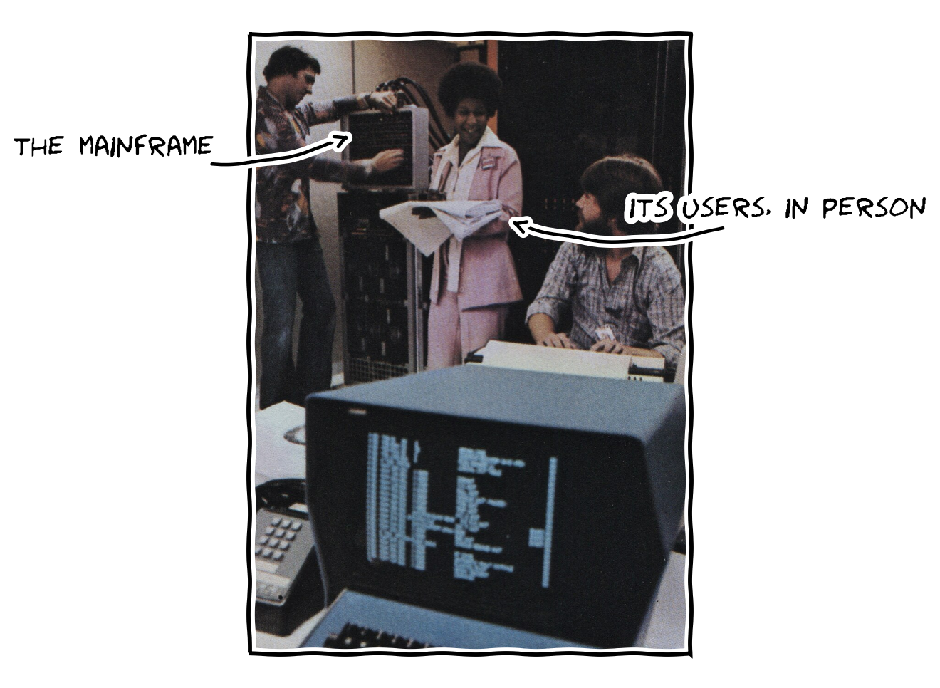
Time-sharing. Many users made one expensive machine cheap per user.
It also explains why open-weight models have not displaced the closed labs as fast as their quality would suggest. You can download a model that rivals the frontier and run it yourself. What you cannot download is the crowd that makes it cheap to serve. So self-hosters pay the empty-plane price, conclude that open weights are expensive, and go back to the API, where someone else’s crowd is subsidizing the utilization. The model was free. The demand was not, and the demand was the real cost driver all along.
Here is the part I find most interesting, and the piece of real engineering I promised at the start. The moat is made of demand, but the amount of demand it takes to cross is not a constant of nature. It is a software number. A serving stack reaches good utilization only once its batch is full, and the batch fills only once enough concurrent requests arrive, so the break-even crowd is set by how large a batch your stack needs in order to run efficiently. Shrink the batch and you shrink the crowd. Every advance that lets a model hit high utilization at a smaller batch, tighter key-value cache paging, better overlap of communication with compute, prefill and decode pulled apart so each runs full, quantization that makes each request cheaper to serve, lowers the number of simultaneous users a deployment needs just to break even. State it exactly and the mechanism is sharp: the frontier lab’s edge is the size of the crowd required to be efficient, and serving-stack engineering attacks that crowd directly, walking the break-even point down toward where a smaller operator can stand. The layout is finished. This floor is wide open, and it is the most valuable engineering in the field right now precisely because every step down it takes is a step out of someone’s moat.
One honest qualification, because the crowd argument assumes a particular kind of demand. It is built for consumer-facing inference, where traffic is large, smooth, and impatient. Other shapes of demand change the arithmetic. A business serving a small but steady and predictable load can fill a right-sized deployment with no crowd at all, because the work arrives on a schedule. Anything that can run offline, a batch or asynchronous job where latency does not matter, can pack its own batches by simply waiting to accumulate enough requests, manufacturing fullness out of patience instead of popularity. Internal enterprise deployments usually look more like the steady case than the bursty one. The moat is real for the spiky, latency-sensitive consumer workload. It is much weaker wherever demand is smooth or can be deferred, and those are not edge cases. They are most of enterprise computing.
scaling laws bend when you have to serve the model
There is one last place the economics reaches back and quietly changes a decision that looks purely technical, which is the choice of how big a model to train at all. The clean rule for spending a training budget balances how large the model is against how much data it sees, and if all you cared about were the loss at the end of training you would follow it. But almost nobody only trains. They train once and serve the result, sometimes billions of times, and serving cost scales with the size of the model you deploy. The moment serving enters the budget the optimum moves: it becomes worth training a smaller model far longer than the clean rule advises, paying more once to own a model that is permanently cheaper to run, because the training bill is paid a single time and the inference bill is paid forever. The same logic drives distillation, where a large and expensive model trains a small and fast one that keeps most of the quality at a fraction of the serving cost. Both are the fixed-cost argument seen from the training side: accept a bigger one-time bill to lower the per-token cost of the thing you will actually keep full.
how full will it be?
A mental model is only worth the decisions it changes, so here is the decision it changes. You were taught to ask whether you can parallelize your workload across N GPUs. The recipes already answered that one: yes, almost certainly, far past what you need. Ask the economic question instead, whether you can keep N GPUs full, and the sizing decision flips. Cluster size should be set by sustained demand, not by model size. A bigger model does not justify more GPUs; enough steady work to fill them does. If demand is small or spiky, fewer GPUs run full beat more GPUs run empty on every axis that matters, and the instinct to add hardware when things feel slow is often exactly backward, because hardware you cannot fill drags down your average utilization and raises your unit cost. Sometimes the right move for a cluster that feels inefficient is to make it smaller.
The break-even hides a number you can compute, and it is worth doing once by hand. Take a 7-billion-parameter model on a single accelerator you rent for about two dollars an hour. When its batch is full it might push on the order of five thousand tokens a second. A small model like this is cheap to serve through an API, call it twenty cents per million output tokens. To beat that price by hosting it yourself you would have to produce two dollars’ worth of tokens every hour, which at twenty cents per million is ten million tokens an hour, a little under three thousand tokens a second held steady. Against a full-batch ceiling of five thousand, that is about sixty percent utilization you have to sustain, all day, through the quiet hours, just to break even. That is where the rough rule comes from that a small model has to stay more than about half full to be worth self-hosting. A larger model moves the floor down rather than up, which is the counterintuitive part: it does more useful work per token and commands a higher API price, so each hour of rent amortizes faster, and the break-even can fall toward ten percent.
The numbers are approximate and the prices move, but the shape is the point. Put in your own rent, your own throughput, and the API price you are measuring against, and your floor falls out. If your honest sustained utilization is below it, the API is not a compromise. It is the cheaper machine, because it runs on someone else’s crowd.
So the next time a scaling decision lands on your desk, do not reach for the parallelism expert first. For every GPU you are about to add, ask what its utilization will be over its life, not at the busy hour but on average, across the dead middle of the night. Because the chip does not care. It draws the same power, depreciates on the same schedule, and bills you for the same hour whether it served a million tokens or none, the way a chartered plane burns the same fuel down the runway whether every seat is taken or the cabin is empty. You can pay, in full, for a thousand empty seats. The parallelism library will fly the plane beautifully. It will not find you the passengers, and finding the passengers was the whole problem from the start.
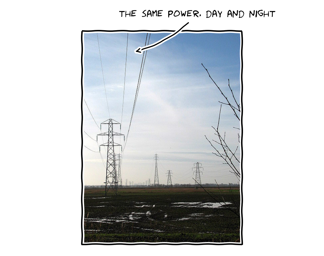
Power lines. The bill comes whether the electricity did anything useful or not.
sources
Sources that shaped this piece: Narayanan et al., Megatron-LM, SC 2021, for the weak-scaling results and the tensor-parallel-within-a-server boundary; Rajbhandari et al., ZeRO, SC 2020, for the sharded data parallelism behind large data-parallel training; Chowdhery et al., PaLM (2022), for the model FLOPs utilization figures across GPT-3, Gopher, Megatron-Turing NLG, and PaLM; Kwon et al., vLLM and PagedAttention, SOSP 2023, for how modern serving stacks raise inference utilization and page the key-value cache; the DatabaseMart vLLM A100 benchmark (2024) for the batch-size throughput numbers; the Introl inference unit-economics analysis for the duty-cycle and break-even figures; Williams, Waterman and Patterson on the roofline model, for the memory-bound framing; Hoffmann et al. (Chinchilla) for compute-optimal scaling, with Vlad Feinberg’s pretraining notes on how inference constraints bend it; and Edward Z. Yang’s writing on SPMD sharding and Megatron mechanics, for the collective-communication picture of why there is essentially one good layout.