Table of Contents
One of the most surprising things in machine learning is that model performance often follows remarkably simple scaling laws. Even a simple model, given more data, more compute, and more parameters, tends to see its error fall in predictable ways. These relationships were mostly observed at first at scales in large research labs, but the underlying ideas are not exclusive to billion-parameter systems. In fact, many of the same patterns emerge in models small enough to train on a laptop.
In this post, we will build a tiny transformer in JAX and derive its scaling behavior from scratch using nothing more than a multiplication table’s worth of two-digit problems, four model sizes, and roughly 300,000 parameters at the largest scale. We will recover several qualitative results that have shaped modern language model training. Even at toy scale, MoE models start pulling ahead for the same fundamental reasons they do in frontier systems.
The experiment runs on a single CPU core in under twenty minutes and doesn’t take much time or compute.
I have also used three papers extensively throughout this post:
- Hoffmann et al. (2022), the Chinchilla paper
- Clark et al. (2022), on scaling laws for routed models
- Krajewski et al. (2024), on fine-grained mixture-of-experts
They provide the correct measurements and support, while our goal is to rebuild the intuition with a toy model small enough to replicate many of the behaviors seen in larger systems. The goal is not to reproduce frontier-scale results exactly, but to understand the underlying ideas end to end.
the task, and why addition is a trap
My first instinct was three-digit addition, the way I suggested in the post. Don’t. Addition is too easy. A 40K-parameter model solves it to a loss of 0.006 and sits there. Once a model has learned the algorithm, a deterministic task has no more information to give, and the scaling curve flattens into a cliff followed by a floor at zero. There is nothing left to fit.
Chinchilla-style laws describe loss approaching an irreducible entropy floor E. On natural text, E is the entropy of language and it is large, so every extra parameter buys a little more of the gap above it, forever. On a deterministic toy task, E = 0, because there is no irreducible uncertainty, so what we are actually measuring is a learnability frontier: how much capacity and how many steps it takes to nail a fixed function. The law keeps the same shape in the unsaturated regime, but the whole model range has to stay unsaturated, or we end up measuring memorization phase transitions instead.
So I switched to two-digit multiplication, aa\bb=cccc, which small transformers find hard, because the carries interact multiplicatively and there is no clean digit-local algorithm. Length-10 character sequences, a vocabulary of twelve. We score only the four answer tokens after the =:
def make_batch(rng, bs):                       # "aa*bb=cccc", score last 4 tokens
    a = rng.integers(0,100,bs); b = rng.integers(0,100,bs); c = a*b
    t = np.empty((bs,10), np.int32)
    t[:,0]=a//10; t[:,1]=a%10; t[:,2]=10       # 10 == '*'
    t[:,3]=b//10; t[:,4]=b%10; t[:,5]=11       # 11 == '='
    t[:,6]=c//1000; t[:,7]=c//100%10; t[:,8]=c//10%10; t[:,9]=c%10
    return jnp.asarray(t)
Data is generated fresh every step, so we are in the single-epoch, infinite-data regime that real pretraining lives in. There is no held-out versus train distinction to fuss over, the model never sees the same batch twice, and tokens seen D is just steps \ batch \ 4. That infinite-data detail is the hinge the dense-versus-MoE comparison swings on.
the model, and the one swap that makes it sparse
The model is the most boring decoder-only transformer we can write: token and learned positional embeddings, pre-norm blocks of causal attention and an MLP, two layers, two heads, nothing tied. The only knob I turn to grow N is d_model. I wrote it in plain JAX with an optax adamw and a warmup-cosine schedule. Flax would be tidier, but I wanted every parameter visible. The swap that turns the MLP into a mixture of experts is smaller than people expect:
def mlp_dense(x, lp):
    return jax.nn.gelu(x @ lp['w1']) @ lp['w2']


def mlp_moe(x, lp):                            # top-1 routing over E experts
    gate = jax.nn.softmax(x @ lp['gate'], -1)  # B,T,E
    top  = jnp.argmax(gate, -1)                # which expert per token
    w    = jnp.max(gate, -1, keepdims=True)    # its gate weight
    h = jax.nn.gelu(jnp.einsum('btd,edf->btef', x, lp['w1']))
    y = jnp.einsum('btef,efd->bted', h, lp['w2'])
    sel = jnp.take_along_axis(y, top[...,None,None], 2).squeeze(2)
    return sel * w
At toy scale I compute all experts and then select, which is wasteful but lets the thing run on a laptop. The accounting is what matters for the scaling story, not the kernel. A top-1 MoE with E experts has roughly E times the MLP parameters but routes each token to one of them, so its active parameter count, the quantity that sets FLOPs per token, is about that of the dense model with the same d_model. Hold that distinction between active and total parameters. It is the whole post.
loss vs data: the family of curves
Train each dense size once for 2000 steps and snapshot the held-out loss at a handful of log-spaced checkpoints. One run gives the entire loss-versus-tokens curve for that size, which is the cheap trick that makes the sweep fit on one core. Four sizes, from 15K to 224K parameters:
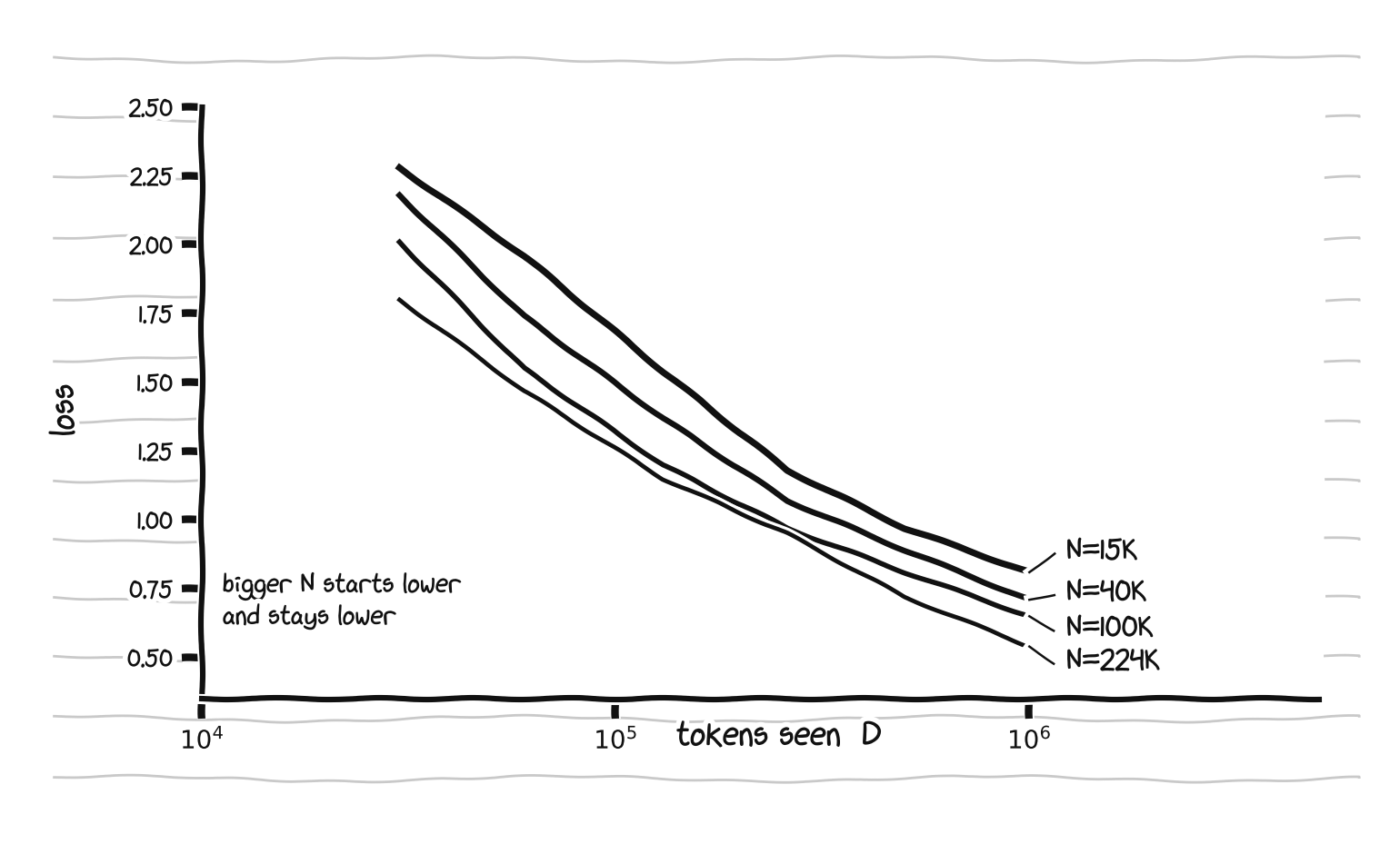
Dense loss versus tokens, one curve per model size. Bigger N starts lower and stays lower.
This is the textbook picture. Bigger models start lower and stay lower. Every curve bends toward its own floor. The gaps between sizes shrink as data grows. Each curve on its own looks like L ≈ B/Dβ sliding down, and the vertical offsets between them are the A/Nα term. That is the entire functional form of
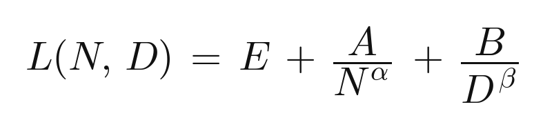
sitting in front of us, decomposed visually into which curve (N) and where on the curve (D).
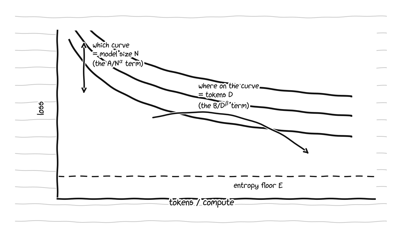
The same law, read off a single curve: vertical position is the model-size term, motion along the curve is the data term.
The three terms each mean something specific, and Hoffmann et al. 2022 name them. E is the loss of an ideal generative process, the entropy of the data itself. A/Nα is the price paid for a finite model that cannot represent the ideal predictor. B/Dβ is the price paid for taking a finite number of optimization steps on a finite sample rather than training to convergence. On our toy, E collapses to zero. On real text it does not, and that single fact is why the law is useful instead of a curiosity.
what the real Chinchilla run actually did
Before deriving anything from the toy, it helps to see how Hoffmann et al. 2022 actually pinned this law down. The toy is a miniature of their third approach, and the method is the point. They trained over 400 models from 70M to 16B parameters and estimated the compute-optimal frontier three independent ways.
The first approach fixes a family of model sizes and varies the number of training tokens, then reads the minimum loss per FLOP off the envelope of all the training curves. The second, the one with the cleanest picture, fixes a set of FLOP budgets and varies model size within each, training every model on exactly the tokens that spend the budget. Plotting final loss against model size at a fixed budget produces a valley:
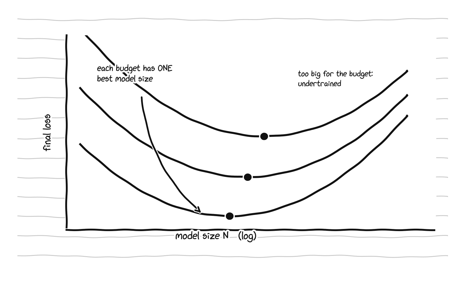
IsoFLOP profiles. For a fixed compute budget the loss has a clear minimum: one best model size per budget.
That valley contains the whole story. For a fixed amount of compute there is a single best model size. Go smaller and the model lacks the capacity to use the budget. Go bigger and there are too few tokens left to train it, so it stays undertrained. The bottom of each valley is the compute-optimal model, and tracing the bottoms across budgets traces the optimal frontier. The third approach fits the parametric form above directly to all the runs with a Huber loss and an L-BFGS solver, which is exactly what we are about to do by hand on the toy.
All three methods agreed. As compute grows, model size and training tokens should grow in almost equal proportion. The fitted exponents put parameter and data scaling at roughly 0.46 to 0.50 each. The closed form they derive for the frontier is
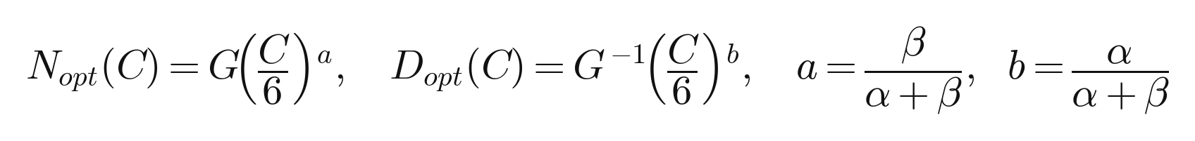
where a and b are built from the two exponents in the loss law. This was a real course correction. Kaplan et al. 2020, working with a fixed learning-rate schedule and a fixed token count, had concluded that a tenfold compute increase should grow the model about 5.5 times and the data only 1.8 times, an exponent near 0.73 on parameters. Hoffmann et al. showed that the fixed schedule was the bug: when the cosine schedule is matched to each run’s token count, the optimal split is close to even.
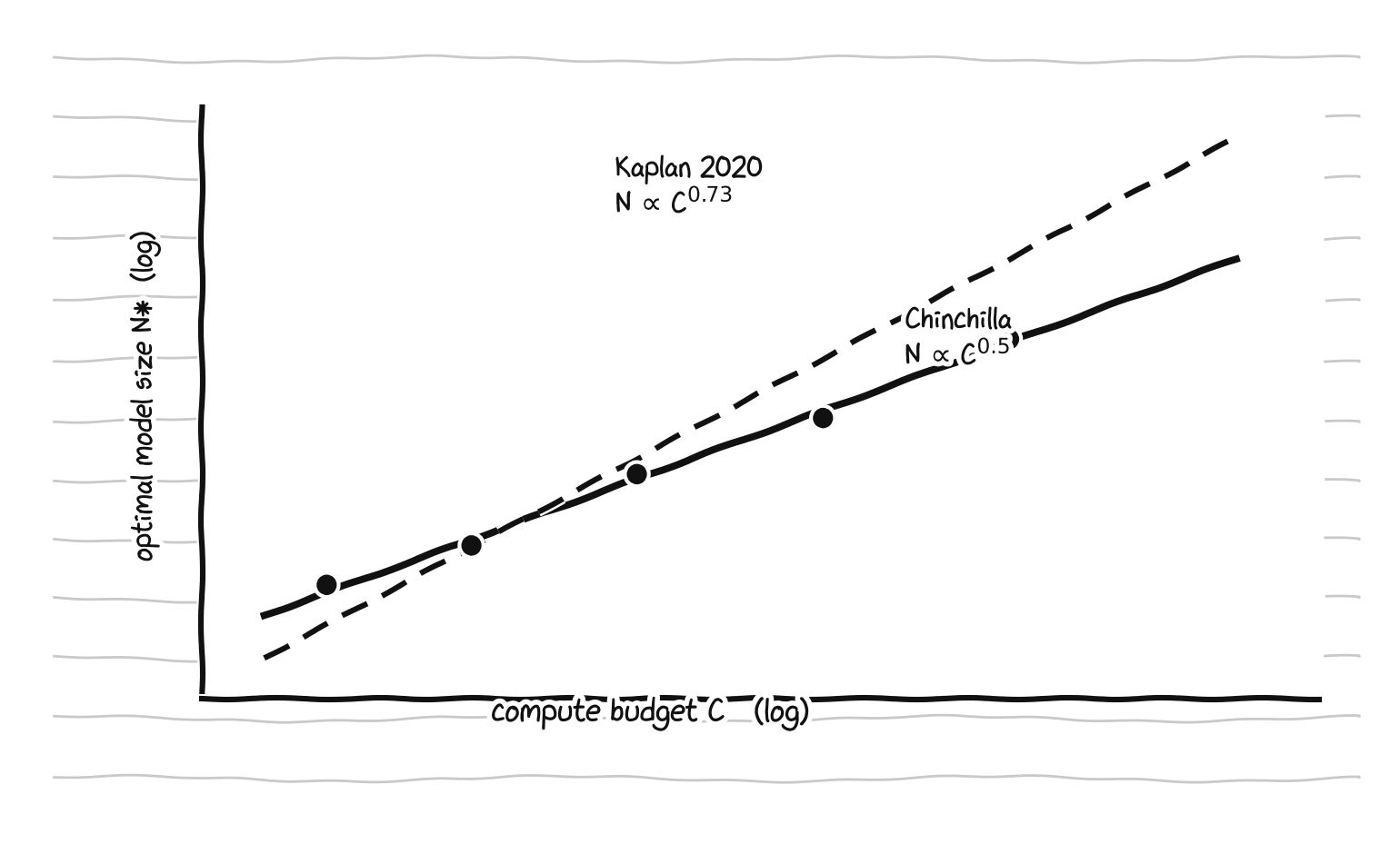
Optimal model size versus compute. Kaplan’s steep line grows the model fast; Chinchilla’s shallower line grows model and data together.
The proof was a model named Chinchilla. They took Gopher’s compute budget, which Gopher had spent on 280B parameters and 300B tokens, and instead trained a 70B model on 1.4 trillion tokens: four times smaller, trained on more than four times the data. Chinchilla beat Gopher, GPT-3, Jurassic-1, and the 530B Megatron-Turing model across the board, while being cheaper to run at inference. The compute-optimal table is blunt about how undertrained the era’s models were. A 175B model wants a budget near 4.4e24 FLOPs and more than 4 trillion tokens to sit on the frontier, far past the 300B tokens everyone was using at the time.
deriving the allocation rule by hand
Back to the toy, where we can now derive that same allocation rule from our own two exponents. Fitting the law is robust least squares on the five parameters (E, A, α, B, β) over the 24 dense (N, D, L) points. I minimize a soft-ℓ1 residual so one noisy run does not drag the exponents around. For the dense model the fit returns E ≈ 0, α ≈ 0.45, β ≈ 0.41.
The E ≈ 0 is the deterministic-task tell I warned about. The fit finds it without being told, which is good. What the two exponents actually prescribe is more interesting. Compute is roughly C ∝ ND, the old six-FLOPs-per-parameter-per-token rule of thumb. To get the most loss reduction for a fixed budget, we minimize L subject to ND held constant:
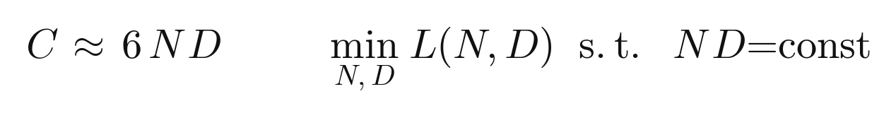
One Lagrange multiplier later, the optimum sets the two reducible terms’ sensitivities equal, and the allocation rule falls out:

Plug in the toy’s dense exponents: β/(α+β) ≈ 0.41/0.86 ≈ 0.47. So the toy says to spend new compute almost evenly between making the model bigger and training it longer, which is almost exactly the Chinchilla finding, reproduced on a task that trains during a coffee break. Hard not to smile at that. The constants are nonsense; the prescription is the real one.
where dense and MoE diverge
Now the same sweep with the top-1, four-expert MoE, and the plot the whole exercise was building toward. I put active parameters on the x-axis, because active parameters are the FLOP-relevant quantity, the honest way to ask what a model cost to run, and compare final loss:
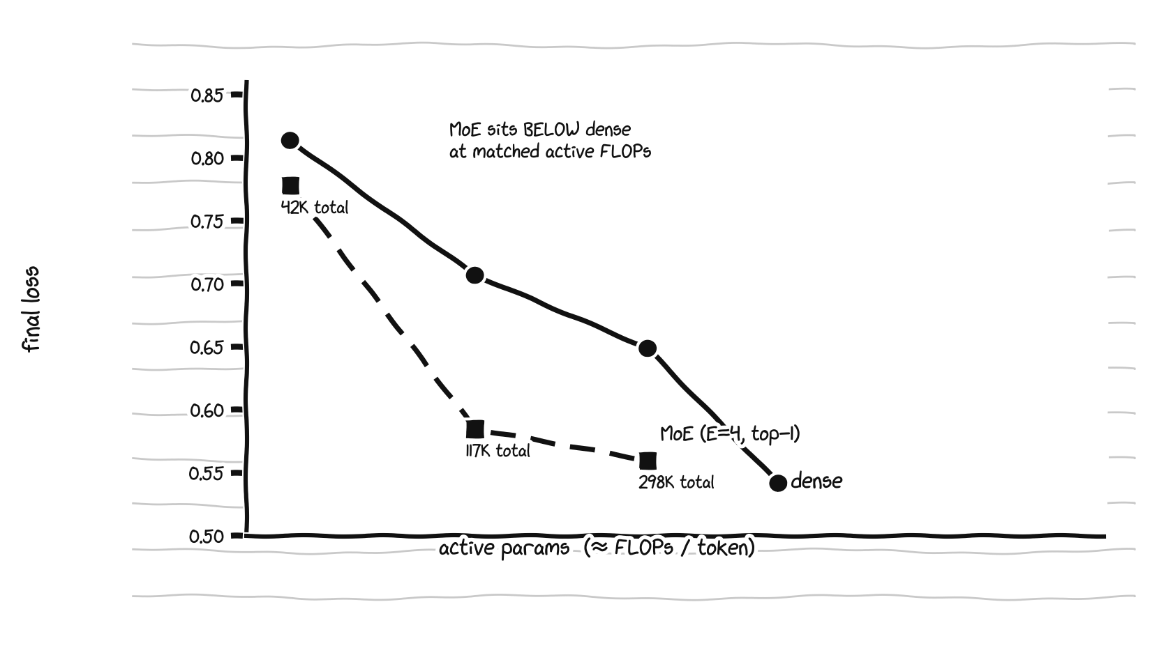
Same active FLOPs, more total parameters. The MoE curve sits below dense at every matched active-parameter budget.
The MoE curve sits under the dense curve at every matched active-parameter budget. Reading off the final losses:
| active params (≈ FLOPs/tok) | dense | MoE (E=4, top-1) | MoE total params |
|---|---|---|---|
| ~15K | 0.814 | 0.778 | 42K |
| ~40K | 0.707 | 0.585 | 117K |
| ~100K | 0.649 | 0.560 | 298K |
Same compute per token, lower loss, because the MoE is quietly carrying about three times the total parameters and the router gets to pick which slice to spend on each token. That is the entire pitch for sparsity in one toy table: parameters are cheap to store, FLOPs are expensive to spend, so decouple them.
Fit the MoE surface on active parameters and the exponents move in exactly the direction the story predicts. The data exponent β ≈ 0.38 barely budges, but the active-parameter exponent α steepens sharply, because each active parameter is now backed by more total capacity, so loss falls faster per active FLOP than for dense. Run that through the allocation rule and the MoE’s compute-optimal frontier tilts toward data: roughly N⋆ ∝ C0.3 instead of dense’s C0.47. When active parameters are this productive, there is no need to grow them as fast, so the marginal compute should go into tokens. The grown-up routed-model papers reach the same conclusion. We just rediscovered it on a single core. I want to be honest that the steep MoE α is pinned by three points, so read it as clearly steeper than dense, not as a number to put in a paper.
the routed-model scaling laws, and the subtlety everyone misses
The grown-up version of that MoE curve is Clark et al. 2022, who trained routed models up to 200B parameters across three routing techniques and fit a law in two variables: the dense base size N and the number of experts E. Their form is bilinear in the logs, with one extra term that does all the interesting work:

The interaction term c log N log E is what does the interesting work. Because c is positive, the benefit of adding experts, captured by the slope b(N) = b + c log N, shrinks as the base model grows. Routing helps a small model a lot and a large model less.
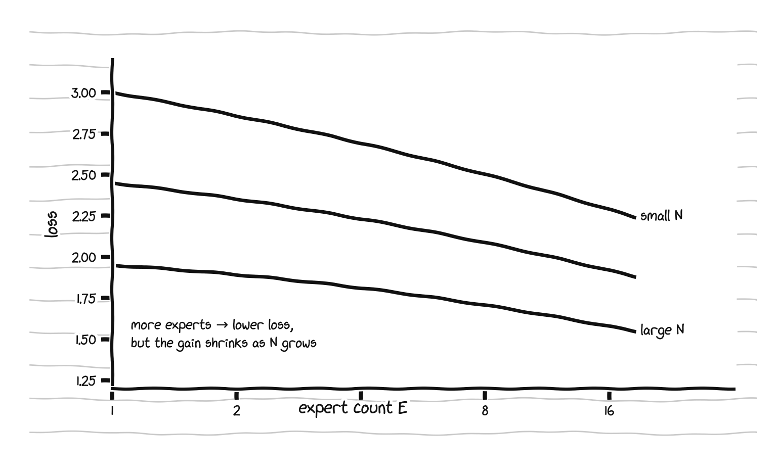
More experts lower the loss, but the gain per expert shrinks as the base model grows. That shrinkage is the interaction term.
Clark et al. push this to its end and compute a cutoff size, the N beyond which adding experts stops helping at all. For their best routing technique it lands near 900B parameters, and for the others closer to 85B. Taken at face value, that says sparsity stops paying off not far above frontier scale, and for a while it was taken to mean exactly that.
Nearly everyone misses what’s actually going on. Clark et al. trained every model on a fixed 130B tokens. That single choice is the same fixed-token mistake that made Kaplan et al. overshoot model size, and it distorts the MoE case even more. A sparse model has more total parameters to fill, so it needs more tokens before it is properly trained, and at a fixed, smallish token budget a large MoE looks undertrained and the gains appear to vanish. The cutoff is real, but it is a statement about 130B tokens, not about sparsity.
granularity, and why MoE is actually always more efficient
Krajewski et al. 2024 reopened the question by relaxing exactly that assumption, letting the token count vary to be compute-optimal for each model, the way Chinchilla did for dense models. Two things flip once you make that fix. First, the conclusion reverses Clark’s. Once training length is chosen properly, a compute-optimal MoE is more efficient than a dense Transformer at every budget they tested, and the gap widens with scale rather than closing. A MoE trained for 1e20 FLOPs matches a dense model given about 20 times the compute, and past 1e25 FLOPs the saving exceeds 40 times.
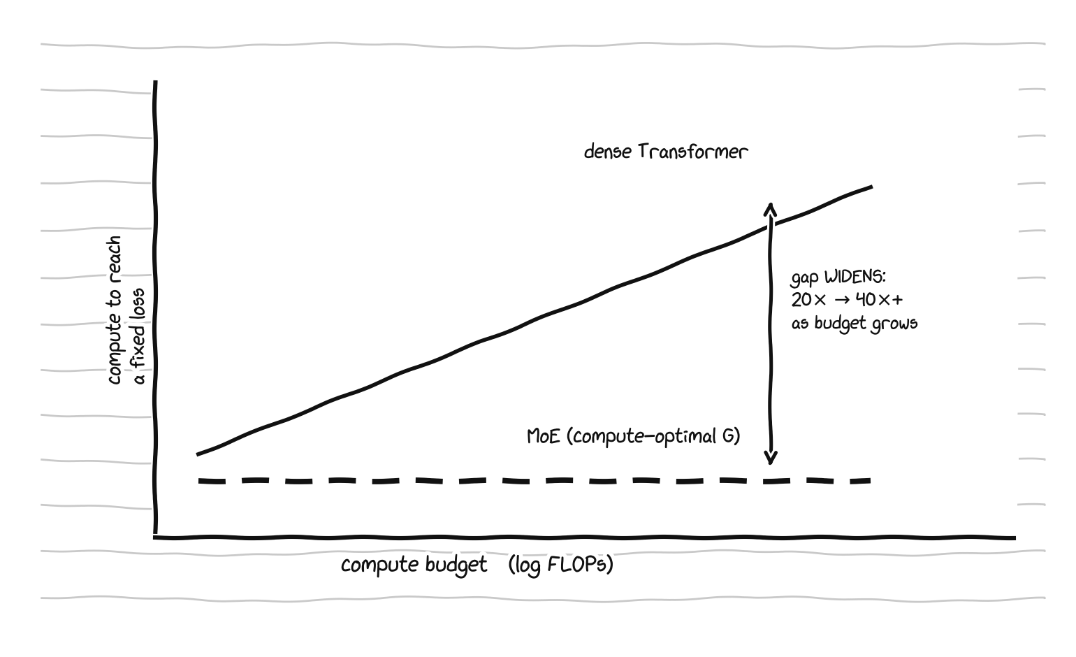
With training length chosen compute-optimally, the MoE efficiency advantage over dense widens as the budget grows.
This is the same hinge the toy quietly relies on. Because the toy generates fresh data every step, it is always in the infinite-data regime, so it never underfeeds the MoE, and the advantage shows up cleanly even at 300K parameters. The fixed-token trap that fooled the fixed-D analysis simply cannot happen on the toy.
Second, Krajewski et al. add a knob the toy’s blunt E = 4 only gestures at: granularity. Instead of forcing each expert to be as wide as the original feed-forward layer, split it into G thinner experts and route each token to G of them, holding the active parameter count fixed:
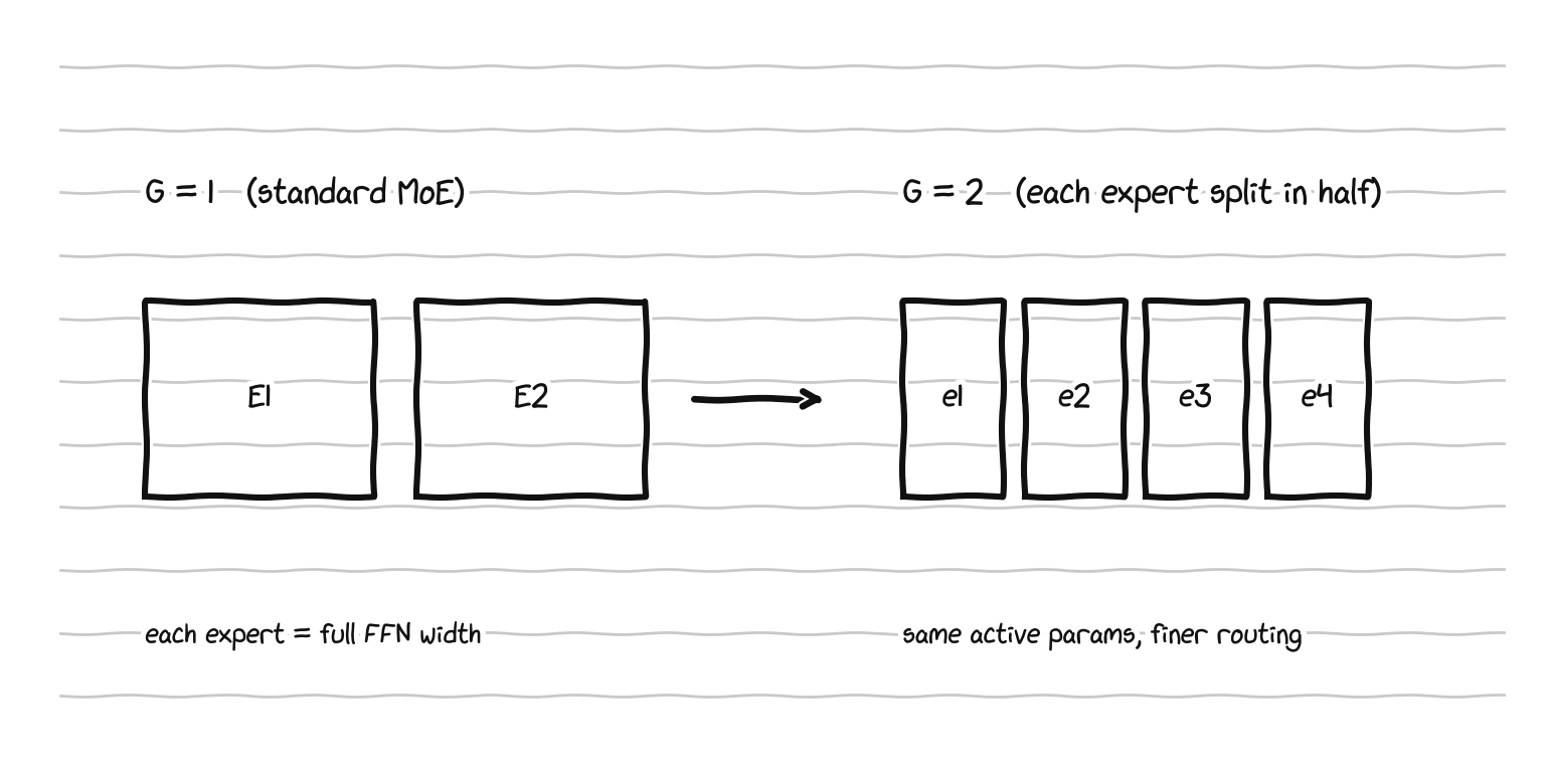
Granularity G splits each expert into G thinner ones; a token is routed to G of them, so active parameters stay constant.
Granularity is just G = d_ff / d_expert, and the number of experts becomes N_expert = G · E. Finer experts give the router a more precise way to map tokens to parameters at no extra active cost, so Krajewski et al. fold granularity into the Chinchilla form as a term that lowers the loss:
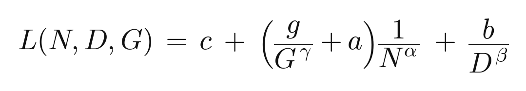
The fitted MoE coefficients land at α ≈ 0.115, β ≈ 0.147, γ ≈ 0.58, with the data term scaling better than dense’s and an irreducible c that matches the dense one, as it must, since the entropy of the data does not care about the architecture. Their main finding: the standard choice of G = 1, one expert per feed-forward width, is almost never compute-optimal, and the optimal G grows with the budget, from around 8 at small scale toward 64 at the largest. The toy’s single jump from dense to E = 4 is the first inch of that curve.
how good is the fit
A scaling law is only as good as its fit. Predicted versus observed loss for both surfaces:
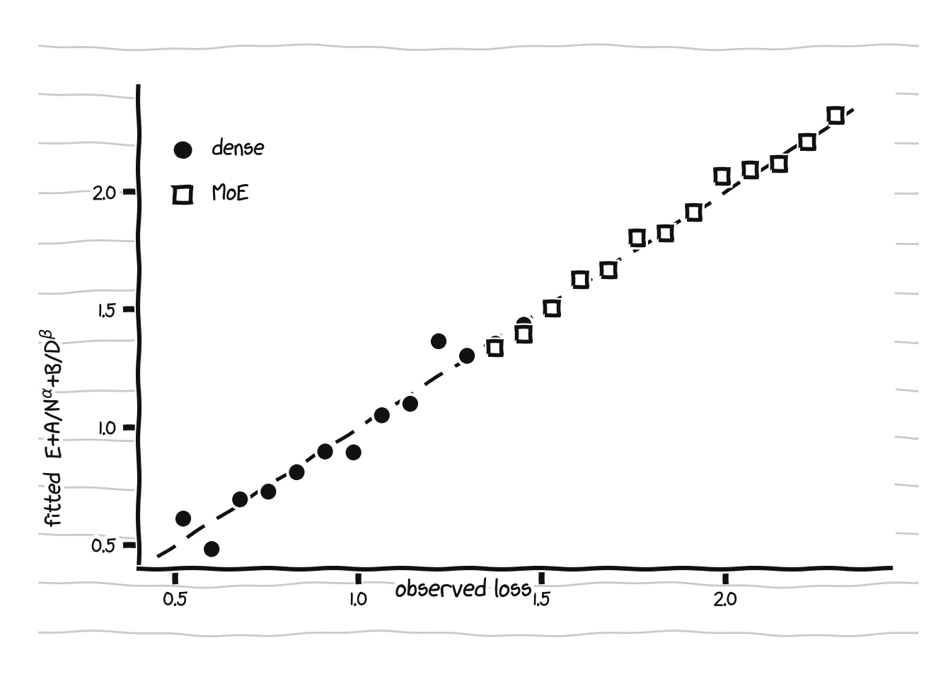
Fitted versus observed loss for the dense and MoE surfaces. Both lie close to the diagonal.
Both lie close to the diagonal, which is the most that 24 dense and a dozen MoE points on one seed can honestly claim. The MoE α in particular rests on three sizes, so it constrains the slope’s sign far better than its value.
what this does and doesn’t show
Everything above is a single seed, four dense and three MoE sizes, two layers, on a deterministic task with no entropy floor, trained for two thousand steps on a CPU. The exponents are illustrative, the E = 0 is an artifact of the toy, and a real sweep would vary depth and width together, use multiple seeds, and push the sizes far enough to constrain α with more than a handful of points. If anyone quotes α = 0.45 as a fact about transformers, I will disavow them.
What it does show is that none of the load-bearing intuition needs scale. The functional form, the visual split into which curve and where on the curve, the Lagrangian that turns two exponents into an allocation rule, the reason MoE sits below dense at matched FLOPs, and the way that reason tilts the optimal frontier, all of it is legible at 300K parameters. The cluster makes the constants trustworthy. It does not make the concepts true. They were true on a laptop the whole time. The one thing the toy cannot show is the fixed-token trap, precisely because it trains in the infinite-data regime, and that trap is what separated Clark’s pessimism from Krajewski’s optimism.
your turn
Two things to try, in ascending order of how much they teach.
First, sweep the number of experts E over {2, 4, 8, 16} at fixed active parameters and watch where the MoE gains saturate. There is a diminishing return here, and the knee is findable by hand. At toy scale, it is the shadow of both Clark’s cutoff and Krajewski’s optimal granularity.
Second, replace the compute-all-experts MoE with a routed implementation using jax.lax.ragged_dot over routed tokens, remeasure cost in wall-clock time instead of active parameters, and redraw the dense-versus-MoE figure with time on the x-axis.
The MoE advantage will shrink because now we are paying for routing and load imbalance. That is the distance between the active FLOP assumption and kernel reality, and I think this is important. Krajewski et al. model this as a per-token routing cost that grows with granularity and eventually eats the gains, which is why their optimal granularity is finite.